Lesson 9: Inequalities

“If people do not believe that mathematics is simple, it is only because they do not realize how complicated life is.” John von Neumann

“Nothing in life is to be feared, it is only to be understood. Now is the time to understand more, so that we may fear less.” Marie Curie

Introduction

In this lesson you embark on a powerful journey to master the art of setting boundaries and exploring what lies between those boundaries. This lesson equips you with tools to solve linear and quadratic inequalities, tackle absolute value challenges, and apply energy and velocity constraints with confidence. Dive into real-world applications like electric circuits, thermal equilibrium, and optimization, where staying within certain bounds unlocks solutions.

We begin by stating that any relationship between quantities where one is potentially larger than another is called an inequality. Inequalities are all about situations where one expression differs from another, unlike the pinpoint equality of equations you conquered previously. Instead of asking “Where does this equal zero?” we’re asking “where is it greater than zero?” or “where is this less than something else?”

Types of Inequalities

For the last three lessons we have been dealing with equations. This gives us a somewhat distorted view of elementary algebra. A frequent problem is to assign bounds to variables where things may no longer be equal, but instead one value may be larger or smaller than another. In this lesson we will show how to solve these kinds of problems, that we will call inequalities. We will then turn to some ramifications of inequalities and several examples. With this kind of backgrounds we will also introduce a lot of concepts of physics. The distinction of an inequality as opposed to an equation, we will-l see that one quantity, say x, is larger than another quantity, say y, we would write x>y. If x is less than y, we write x<y. It is also possible that x can either be greater than or equal to y, we write x >=y. Then we can also have x as less than or equal to y, x<=y.

Solving Linear Inequalities

We now begin our examination of inequalities with the simplest type. In direct analogy to linear equations, if we replace the equals sign with some kind of inequality symbol, then we have a linear inequality. For example,

(9.1)

Solving this is a lot like solving equations, except we have replaced = by <. We start by adding 3 to each side.

(9.2)

Then we divide by 2,

(9.3)

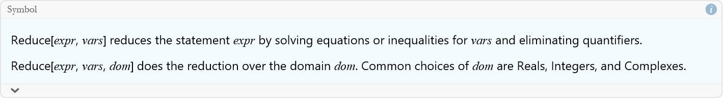
That’s it—x can be any number less than 4.  WL confirms the answer in (9.3). We use the Reduce command.

We can flip the direction of the inequality by multiplying both sides by a negative number, -x>-4. For example, we multiply both sides of (9.1) by -1,

(9.4)

We start by subtracting 3 from each side.

(9.5)

Then we divide by 2,

(9.6)

Terms and Definitions

Term/Definition 9.1 Inequality: A mathematical statement that compares two expressions using symbols > (greater than), < (less than), ≥ (greater than or equal to), or ≤ (less than or equal to).

Term/Definition 9.2 Linear inequality: An inequality where the variable(s) are raised only to the power of 1 (no higher powers); analogous to linear equations but with inequality symbols.

Term/Definition 9.3 Single-variable linear inequality: A linear inequality with only one unknown variable (e.g., 2x - 3 < 5).

Term/Definition 9.4 Reduce[] (Wolfram Language function): A command that solves equations or inequalities symbolically, reducing them to a form that describes the solution set (e.g., x < 4).

Term/Definition 9.5 Solution set: The collection of all values that satisfy an inequality (e.g., all x < 4).

Term/Definition 9.6 Flipping the inequality: Reversing the direction of the inequality symbol when multiplying or dividing both sides by a negative number (e.g., -x > -4 becomes x < 4).

Assumptions (the implicit beliefs the author relies on)

Assumption 9.1: Inequalities are a natural extension of equations, using >, <, ≥, ≤ instead of =.

Assumption 9.2: Linear inequalities can be solved using the same balancing principle as linear equations.

Assumption 9.3: Identical operations on both sides preserve the inequality (except when multiplying/dividing by negative, which flips the direction).

Assumption 9.4: The solution set for linear inequalities is typically an interval or half-line (e.g., x < 4 means all x less than 4).

Assumption 9.5: Wolfram Language Reduce[] reliably solves linear inequalities and returns the solution set.

Assumption 9.6: Negative coefficients or constants require careful sign handling (flipping when multiplying/dividing by negative).

Assumption 9.7: Solving inequalities is foundational for understanding ranges, constraints, and physical limits.

Principles

Principle 9.1: Inequalities compare expressions: x > y, x < y, x ≥ y, x ≤ y.

Principle 9.2: Verify solutions by substituting test values from the solution set into the original inequality.

Exercise 9.1: Begin with Term/Definition 9.1 and copy it into your notebook. Reflect on its meaning for a few minutes. Note any thoughts that come to mind. How would you explain this to someone sitting in front of you. Write this down. Then do this for each term/definition, assumption, and principal.

Exercise 9.2: Solve
a) 3 v - 6<9 for v.
b) 2 T - 4<10 for T.
c) -4 f +8<0 for f.
d) 5 x -10<15 for x.
e) -3 I +9<6 for I.

Linear Inequalities on a Number Line

Solving linear inequalities gives us a solution set (e.g., x<4 for our example in (9.3)), it’s often helpful to visualize this set to better understand the range of possible values. This is especially useful in theoretical physics, where inequalities describe constraints, such as a particle’s position or speed within a certain range. In this section, we’ll learn how to represent the solutions of linear inequalities on a number line, a simple yet powerful tool for visualizing intervals.

Recall from lesson 3 that a number line is a horizontal line where each point represents a number. Negative numbers are to the left of zero, and positive numbers are to the right. To show the solution of a linear inequality, we shade the region of the number line where the inequality holds true and mark boundary points with circles to indicate whether they’re included.

Here’s how we represent different inequalities. For example, given,

(9.7)

you shade all numbers to the left of a. Use an open circle at a to show that it is not included.

For the example,

(9.8)

you shade to the left of a. Use a closed circle at a to show that it is included.

For the example,

(9.9)

you shade all numbers to the right of a. Use an open circle at a to show that it is not included.

For the example,

(9.10)

you shade to the right of a. Use a closed circle at a to show that it is included.

Let’s visualize some solutions. We begin with,

(9.11)

The work flow is like this:

Draw a number line with a scale.

Place an open circle at 2, indicating 2 is not included.

Draw an arrow pointing left to show all numbers less than 2.

Here is what it looks like.

Next we try

(9.12)

Next, we try,

(9.13)

Here, the work flow is a bit different:

Draw a number line with a scale.

Place a closed circle at -1, indicating -1 is included.

Draw an arrow pointing right to show all numbers greater than or equal to -1.

It looks like this.

Some inequalities, called compound inequalities, describe a range between two values, like a<x<b. For example, consider the solution −1<x≤2. Here is the workflow for this:

Draw a number line with a scale.

Place a open circle at -1, indicating -1 is not included.

Place a closed circle at 2, indicating that it is included.

Draw a line between the circles.

Here is what it looks like.

As introduced in Chapter 5, Wolfram Language is a powerful tool for symbolic computation. You can use it to visualize inequalities on a number line with the NumberLinePlot function. For example, to plot x<2, we write:

We can place the inequality on the line itself if we use Spacings->0.

For a compound inequality like −1<x≤2, we write,

Terms and Definitions

Term/Definition 9.7 Open circle (on number line): A circle at a boundary point indicating the value is not included (used for < or >).

Term/Definition 9.8 Closed circle (on number line): A filled circle at a boundary point indicating the value is included (used for ≤ or ≥).

Term/Definition 9.9 Shaded region (on number line): The part of the line indicating the solution set (all values satisfying the inequality).

Term/Definition 9.10 Compound inequality: An inequality combining two or more conditions (e.g., -1 < x ≤ 2), describing a range between two values.

Term/Definition 9.11 NumberLinePlot[] (Wolfram Language function): A command that plots inequalities on a number line, showing shaded regions, open/closed circles, and arrows.

Term/Definition 9.12 Spacings (option in NumberLinePlot): An option to control spacing or style (e.g., Spacings → 0 places inequality directly on the line).

Assumptions (the implicit beliefs the author relies on)

Assumption 9.8: Linear inequalities have solution sets that are intervals or half-lines on the number line.

Assumption 9.9: The number line is a clear, intuitive way to visualize inequality solutions.

Assumption 9.10: Open circles are used for strict inequalities (<, >); closed circles for inclusive inequalities (≤, ≥).

Assumption 9.11: Arrows indicate the direction of the solution set (left for less than, right for greater than).

Assumption 9.12: Compound inequalities describe bounded ranges (e.g., -1 < x ≤ 2).

Assumption 9.13: Wolfram Language NumberLinePlot accurately visualizes inequalities with proper circles, shading, and arrows.

Principles

Principle 9.3: Represent linear inequalities on a number line: shade the solution set, use open/closed circles at boundaries, and arrows for direction.

Principle 9.4: For x < a: shade left of a, open circle at a.

Principle 9.5: For x ≤ a: shade left of a, closed circle at a.

Principle 9.6: For x > a: shade right of a, open circle at a.

Principle 9.7: For x ≥ a: shade right of a, closed circle at a.

Exercise 9.3: Begin with Term/Definition 9.7 and copy it into your notebook. Reflect on its meaning for a few minutes. Note any thoughts that come to mind. How would you explain this to someone sitting in front of you. Write this down. Then do this for each term/definition, assumption, and principal.

Exercise 9.4:
a) Solve 4v-8<12 for v.
b) Solve 3T+5<14 for T.
c) Solve -5f+10<0 for f, note the sign flip.
d) Solve 2x-6<4 for x, then plot the solution region.
e) Solve -2I+7<3 for I.

Linear Inequalities on a Coordinate Plane

How do we plot an inequality in two-dimensions? We use Plot with a new option.

If it is greater than, we use Filling->Top.

Terms and Definitions

Term/Definition 9.13 Linear inequality (in two dimensions): An inequality of the form a x + b y + c < 0 (or >, ≤, ≥), defining a half-plane in the coordinate plane.

Term/Definition 9.14 Half-plane: One side of a line in the Cartesian plane, representing all points that satisfy the inequality.

Term/Definition 9.15 Boundary line: The line a x + b y + c = 0; the edge separating the two half-planes.

Term/Definition 9.16 Solid line (in inequality graph): A solid boundary line indicates the inequality includes the line (≤ or ≥).

Term/Definition 9.17 Dashed line (in inequality graph): A dashed boundary line indicates the inequality excludes the line (< or >).

Term/Definition 9.18 Shaded region: The filled area on one side of the boundary line showing all points (x, y) that satisfy the inequality.

Term/Definition 9.19 Filling (option in Plot): A Plot option in Wolfram Language to shade one side of the curve (e.g., Filling → Bottom shades below the line, Filling → Top shades above).

Assumptions (the implicit beliefs the author relies on)

Assumption 9.14: Linear inequalities in two variables define half-planes in the Cartesian coordinate plane.

Assumption 9.15: The boundary line is included for ≤ or ≥ (solid line) and excluded for < or > (dashed line).

Assumption 9.16: Shading one side of the line represents the solution set (all (x, y) pairs satisfying the inequality).

Assumption 9.17: Wolfram Language Plot[] with Filling accurately visualizes the solution region of a linear inequality.

Assumption 9.18: Filling → Bottom shades below the line; Filling → Top shades above (direction depends on inequality).

Principles

Principle 9.8: Graphing linear inequalities reveals solution regions — crucial for constraints in physics (feasible regions, bounds).

Principle 9.9: Practice plotting by hand first (boundary line, test point, shade), then verify with WL Plot + Filling.

Exercise 9.5: Begin with Term/Definition 9.13 and copy it into your notebook. Reflect on its meaning for a few minutes. Note any thoughts that come to mind. How would you explain this to someone sitting in front of you. Write this down. Then do this for each term/definition, assumption, and principal.

Exercise 9.6:
a) Solve 5v+3<18 for v, then plot the solution.
b) Solve 2P-7<18 for P, then plot the solution.
c) Solve -3f+9<6 for f, then p[lot the solution.
d) Solve 3x+2<11 for x, then plot the solution region.
e) Solve -4Q+12<8 for Q, then plot the solution.

Solving Quadratic Inequalities

Any inequality that involves a quadratic expression is called a quadratic inequality. In this section, we’ll learn how to solve quadratic inequalities and represent their solutions on a coordinate plane, building on the skills from Lesson 7 (Quadratic Equations) and the linear inequality techniques from earlier in this lesson.

A quadratic inequality compares a quadratic expression to some quantity (or another expression) using inequality symbols (<,>,≤,≥). Here are some examples,

(9.14)

(9.15)

(9.16)

The solution to a quadratic inequality is typically a set of intervals on the number line, unlike quadratic equations, which have at most two solutions. Our goal is to find all values of x that make the inequality true.

Solving a quadratic inequality involves finding the roots of the corresponding quadratic equation, determining the behavior of the quadratic function, and testing intervals to identify where the inequality holds. Here’s the process:

Rewrite the inequality in the form   (or <0,≤0,≥0). If necessary, move all terms to one side.

Find the roots of the associated quadratic equation .

Plot the roots on a number line. These roots divide the number line into intervals.

Test a point in each interval to determine where the quadratic expression is positive (>0) or negative (<0).

Determine the solution based on the inequality symbol, including or excluding the roots as needed (≤,≥, include roots or <,> exclude them).

Represent the solution on a number line, as described in the previous section.

As an example let’s solve the  quadratic inequality .

The inequality is already in the form , .

Find the roots of the quadratic equation . This gives us x={2,3}.

Plot the roots on a number line.

Note the gap.

Test a point in each interval to determine where the quadratic expression is positive (>0) or negative (<0). First we try: x=1 ⇒ 12−5⋅1+6=2>0 is True. Then we try x = 2.5 ⇒ 6.25 - 12.5 + 6 = -0.25 > 0 is False. This is why there is no solution in the central gap. Then we try x=4 ⇒ 16 -20 +6 = 2 > 0 is True.

The solution is positive where x<2 or when x>3.

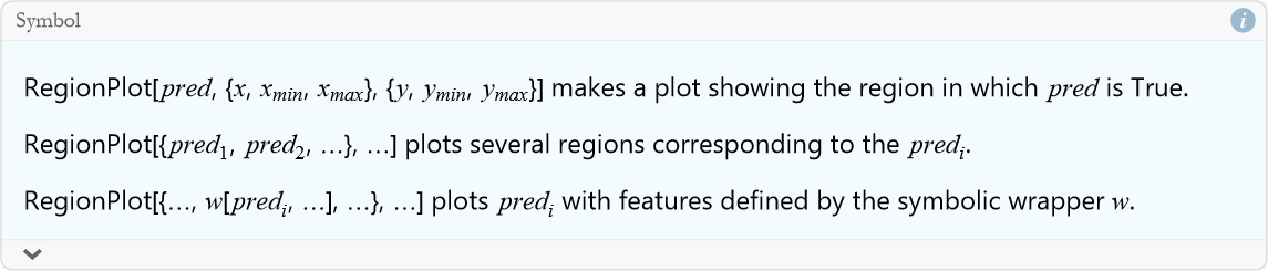
While number lines show solutions in one dimension, quadratic inequalities can also be visualized in a coordinate plane, where we plot the quadratic expression and identify regions where the inequality holds. This is similar to how we have explored linear inequalities in a coordinate plane in the previous section, but quadratics produce parabolas, leading to more complex regions. In Wolfram Language we introduce RegionPlot.

For our example we write.

We can also write,

Terms and Definitions

Term/Definition 9.20 Quadratic inequality: An inequality involving a quadratic expression (e.g., etc.).

Term/Definition 9.21 Sign chart (or sign analysis): A method of testing the sign (+ or –) of the quadratic expression in each interval determined by the roots.

Term/Definition 9.22 Test point: A chosen value in each interval between roots to determine whether the quadratic expression is positive or negative in that interval.

Term/Definition 9.23 RegionPlot (Wolfram Language function): A command that plots the region in the coordinate plane where a predicate (inequality) is true (e.g., RegionPlot[x² - 5x + 6 > 0, {x, -5, 5}, {y, -10, 10}]).

Assumptions (the implicit beliefs the author relies on)

Assumption 9.19: Quadratic inequalities can be solved by first finding the roots of the associated quadratic equation .

Assumption 9.20: The roots divide the number line into intervals where the quadratic expression does not change sign.

Assumption 9.21: Testing a single point in each interval reveals the sign of the expression throughout that interval.

Assumption 9.22: The inequality holds where the expression is positive (> 0) or negative (< 0), depending on the symbol; equality at roots for ≤ or ≥.

Assumption 9.23: Wolfram Language RegionPlot accurately visualizes the solution region in the coordinate plane.

Principles

Principle 9.10: Solve quadratic inequalities by:

Rewrite in standard form (or <, ≥, ≤).

Solve the equation to find roots.

Plot roots on number line to divide into intervals.

Test a point in each interval to determine sign (+ or –).

Include roots for ≥ or ≤; exclude for > or <.

Principle 9.11: Roots are critical: they are boundary points where the expression changes sign (or touches zero).

Principle 9.12: The solution set is the collection of intervals where the inequality holds true.

Exercise 9.7: Begin with Term/Definition 9.20 and copy it into your notebook. Reflect on its meaning for a few minutes. Note any thoughts that come to mind. How would you explain this to someone sitting in front of you. Write this down. Then do this for each term/definition, assumption, and principal.

Exercise 9.8:
a) Solve for t, then plot the solution.
b) Solve for x, then plot the solution.
c) Solve for v, then p[lot the solution.
d) Solve for f, then plot the visualize the region.
e) Solve for x, then plot the solution.

A General Solution Strategy

Inequalities, whether describing the safe operating range of a spacecraft or the stability of a pendulum, are powerful tools in physics and mathematics. A general strategy for solving any inequality—be it polynomial, rational, or absolute value—ensures clarity and consistency. This approach leverages algebraic techniques and computational tools like the Wolfram Language to find and visualize solution regions, empowering you to tackle physical problems with confidence.

Step 1: Identify the Inequality and Its Context

Determine the inequality’s form (e.g., polynomial, rational, absolute value) and its physical significance. For instance, an inequality like ∣x−2<1 might define a region where a particle stays within a certain distance from a point. Clarify whether the solution requires a numerical interval, a graphical region, or a physical interpretation.

Step 2: Standardize the Inequality

Rewrite the inequality with zero on one side to simplify analysis. For example, transform into . This form highlights the expression to analyze and prepares it for solution.

Step 3: Find Critical Points

Solve the associated equation (set the expression equal to zero) to identify boundaries where the inequality may change its behavior. For a rational inequality like , solve , yielding x=1. Also, identify points where the expression is undefined (e.g., x=−2 for the denominator). Use the Wolfram Language for precision:

Check for undefined points separately.

Step 4: Divide into Intervals

Use critical points (roots and undefined points) to split the number line into intervals. For , the critical points x=1 and x=−2 create intervals: (−∞,−2), (−2,1), and (1,∞). Test a point in each interval to determine where the inequality holds. For example, test x=0:

Since , this tells us that the interval (-2,1) is not part of the solution.

Step 5: Visualize the Solution

Graphical representations clarify solution regions, especially for complicated inequalities. Plot the expression and identify where it satisfies the inequality (e.g., above or below zero). For a polynomial like , visualize the function:

This plots the solution curve for   and fills the region between that curve and the horizontal axis,  highlighting where . For two-variable inequalities, such as , which might represent a particle confined within a circular region of radius 2 (e.g., in a magnetic field), use:

Step 6: Check Boundary Conditions

Verify whether boundaries are included (e.g., ≤ vs. <) and ensure the solution fits the inequality’s structure. For the polynomial inequality , use:

This confirms the regions where the inequality is true, such as numbers less than - or greater than . Check that the solution fits the physical context, like a valid range of positions (assuming this is a physics problem, and not a purely mathematical one).

Step 7: If this is a Physics Problem, Connect the Solution to the Physics

At the heart of theoretical physics we have two approaches to solving problems. Both are very similar in general, though widely differing in methodology. Mathematical physics turns a physics problem into a mathematics problem. You solve the mathematics problem and then connect your solution back to the physics problem. Computational; physics turns your physics problem into a computer coding problem. You write the code and produce the output, then attempt to interpret the output in the context of your original physics problem.

This set of six or seven steps works for any inequality, from simple linear to complicated rational forms. Use computational tools to boost your accuracy and practice applying solutions to physics problems, building your skills as a physics explorer.

Terms and Definitions

Term/Definition 9.24 Critical points: The roots of the associated equation (where expression = 0) and points where the expression is undefined (e.g., denominators = 0).

Term/Definition 9.25 Intervals: The regions on the number line or coordinate plane divided by critical points; the expression does not change sign within each interval.

Assumptions (the implicit beliefs the author relies on)

Assumption 9.24: All inequalities (linear, quadratic, rational, etc.) can be solved using a systematic, step-by-step strategy.

Assumption 9.25: Critical points (roots and undefined points) divide the domain into intervals where the expression does not change sign.

Principles

Principle 9.13: General solution strategy for inequalities:

Identify inequality and context (physical meaning, domain).

Standardize: rewrite with zero on one side.

Find critical points (roots of = 0, undefined points).

Divide domain into intervals using critical points.

Test point in each interval to determine sign.

Include/exclude boundaries based on inequality symbol.

Visualize with RegionPlot or Plot + Filling.

Connect solution to physics (constraints, meaning).

Exercise 9.9: Begin with Term/Definition 9.24 and copy it into your notebook. Reflect on its meaning for a few minutes. Note any thoughts that come to mind. How would you explain this to someone sitting in front of you. Write this down. Then do this for each term/definition, assumption, and principal.

Exercise 9.10:
a) Solve for t, then plot the solution.
b) Solve for x, then plot the solution.
c) Solve for v, then plot the solution.
d) Solve for f, then plot the visualize the region.
e) Solve for x, then plot the solution.

Absolute Values

Recall that the absolute value of a number measures its distance from zero on the number line, ignoring direction. For example, the distance from -3 to 0 is the same as from 3 to 0, so both have an absolute value of 3. This section introduces absolute values in terms of inequalities, their properties, and how to solve expressions involving them.

The absolute value of a quantity x is written |x|, and we can define it precisely.

(9.17)

We can write this in a more elegant way,

(9.18)

For instance, |5| = 5, and |-5| = -5 · (-1) = 5. In physics, if a particle moves 5 meters left or right from a starting point, its displacement’s absolute value is |5| = 5 or|-5| = 5, focusing on the distance traveled.

Absolute values follow several key rules:

Absolute values are never negative. This makes sense if you think of it as the distance from zero. A distance can be zero, but it can’t ever be less than zero; what would that even mean?

An absolute value of a negative number is always equal to the absolute value of the positive counterpart, |-x|=|x|.

The absolute value of a product is the product of the absolute values |x·y|=|x|·|y|.

These properties help simplify expressions.

Equations involving absolute values, like |x - 2| = 3, arise in physics, for example when you find positions equidistant from a point. This equation could represent a particle 3 meters away from a reference point at x=2. We would write this|x - 2| = 3:

Recognize that|x - 2| = 3 means x−2=3 or x−2=−3, since the expression inside the absolute value can be positive or negative.

Solve each case

(9.19)

(9.20)

Check solutions by substituting back.

(9.21)

(9.22)

Thus, the solutions are x=5 or x=-1, meaning that the particle is at position 5 or -1 on the number line.

In WL we would write the code:

Note the warning message.

Let’s see what happens when we use Reduce, as suggested.

Note that the only time when the solution is not 5 or -1 is when the expression involves imaginary numbers.

Graphs clarify how absolute values work. The equation∣y = |x - 2| forms a V-shaped graph with its vertex at x=2, since|x - 2| measures the distance from x to 2. To solve|x - 2| = 3, find where the graph equals 3. To plot it:

This shows the V-shape intersecting y=3 at x=−1 and x=5, matching the solutions. In physics, this graph could represent the distance a particle is from a fixed point over time.

Terms and Definitions

Term/Definition 9.26 Absolute value (symbol |x|): The distance of a number x from zero on the number line, always non-negative; ignores direction. Absolute value definition:  |x| = x if x ≥ 0, |x| = -x if x < 0, (piecewise definition)

Term/Definition 9.27 Complex conjugate (symbol z*): For z = a + b i, the conjugate is a - b i (flips the sign of the imaginary part).

Term/Definition 9.28 Conjugate product: The product , always a real, non-negative number.

Term/Definition 9.29 V-shaped graph: The graph of y = |x - c|; forms a V with vertex at (c, 0), reflecting distance from c.

Assumptions (the implicit beliefs the author relies on)

Assumption 9.26: Absolute value measures distance from zero (or from a point), always ≥ 0.

Assumption 9.27: Absolute value equations like |x - c| = k represent points equidistant from c (two solutions symmetric around c).

Assumption 9.28: Absolute value is never negative (distance cannot be negative).

Assumption 9.29: Wolfram Language Abs[] correctly computes absolute value for real and complex numbers.

Principles

Principle 9.14: Property: |x·y| = |x|·|y| (product of absolute values).

Principle 9.15: Property: |-x| = |x| (absolute value ignores sign).

Principle 9.16: Absolute value equations like |x - c| = k have two solutions (unless k = 0, one solution).

Exercise 9.11: Begin with Term/Definition 9.26 and copy it into your notebook. Reflect on its meaning for a few minutes. Note any thoughts that come to mind. How would you explain this to someone sitting in front of you. Write this down. Then do this for each term/definition, assumption, and principal.

Exercise 9.12:
a) Solve |v-3|<2 for v, then plot the solution.
b) Solve |x+1|<0 for x, then plot the solution.
c) Solve |f-5|<3 for f, then plot the solution.
d) Solve |x-2|<5 for x, then plot the solution.
e) Solve |I+2|<6 for I, then plot the solution.

Energy Inequalities

In physics, energy governs how systems behave. Inequalities help us understand the conditions under which a system has enough energy—or too much—for certain outcomes. This section explores how inequalities model energy constraints, using the tools you’ve learned to analyze physics problems.

Energy inequalities describe ranges of values where a system’s energy meets specific requirements. For example, in mechanics, the kinetic energy of an object, , where m is mass and s is speed, might need to exceed a certain threshold to overcome friction. Inequalities let us find the speeds, positions, or times that satisfy these conditions, connecting mathematics to physical phenomena.

Suppose a vehicle of mass m=1000 kg needs kinetic energy greater than 50,000 J to climb a hill. The kinetic energy is , so the inequality is

(9.23)

We simplify both sides by dividing by 500,

(9.24)

This is a quadratic inequality. Using the general strategy from above, we solve the associated equation ,

(9.25)

We test these regions around these points; numbers less than -10, between -10 and 10, and then greater than 10. For s=15,

(9.26)

For s=0,

(9.27)

For s=-15,

(9.28)

The inequality holds for speeds less than -10 or greater than 10. Since speed’s direction matters in this context (e.g., moving forward or backward), both ranges are relevant. We can use the Wolfram Language to confirm our solutions:

We can also graph this.

Next we consider a spring with potential energy , where we have the spring constant k=200 units and x is the displacement from equilibrium. Suppose the spring’s potential energy must be less than 50 units to avoid damage. The inequality is:

(9.29)

We solve the equation ,

(9.30)

Now we test the different regions (numbers less than -0.707, between -0.707 and 0.707, and greater than 0.707). For x=0

(9.31)

For x=1

(9.32)

So, the inequality holds for values between -0.707 and 0.707. We can verify this using WL:

This confirms the solution is approximately -0.707 < x < 0.707. We can plot this situation:

So, as we have seen energy inequalities define the boundaries of physical systems. Practice solving them to understand when a rocket has enough energy to escape Earth or when a pendulum stays within safe limits are only two examples of a vast landscape that these problems open up. Use Wolfram Language to check solutions and visualize regions, making energy concepts tangible as you explore the physics of the universe.

Terms and Definitions

Term/Definition 9.30 Energy inequality: An inequality that defines ranges or bounds on a system's energy (e.g., kinetic energy > threshold, potential energy < limit) to meet physical conditions or safety constraints.

Term/Definition 9.31 Total mechanical energy (symbol E): The sum of kinetic and potential energies in a system; E = T + U.

Term/Definition 9.32 Threshold: A minimum or maximum energy value required for a process to occur (e.g., kinetic energy > 50,000 J to climb a hill).

Term/Definition 9.33 Epilog (option in Plot): Adds extra graphics (e.g., dashed lines, thresholds) to a plot for emphasis.

Assumptions (the implicit beliefs the author relies on)

Assumption 9.30: Energy in physical systems can be modeled as kinetic + potential (mechanical energy), with total E conserved in isolated systems.

Assumption 9.31: Energy inequalities define safe, feasible, or required operating ranges (e.g., enough kinetic energy to overcome friction, potential energy below damage limit).

Principles

Principle 9.17: Energy inequalities constrain physical systems: define ranges where energy meets requirements (e.g., T > threshold, U < limit).

Principle 9.18: Total mechanical energy E = T + U is conserved in isolated systems (no friction, etc.).

Principle 9.19 Conservation of energy: The principle that total mechanical energy E remains constant in an isolated system (no non-conservative forces like friction).

Exercise 9.13: Begin with Term/Definition 9.30 and copy it into your notebook. Reflect on its meaning for a few minutes. Note any thoughts that come to mind. How would you explain this to someone sitting in front of you. Write this down. Then do this for each term/definition, assumption, and principal.

Exercise 9.14:
a) Given a 1200 kg vehicle needing kinetic energy greater than 60,000 J to climb a hill, derive and solve the inequality for speed s. Use Solve and Plot to visualize the solution region.
b) For a spring with k=300 units and a maximum potential energy of 75 J, determine the displacement range x where . Test intervals and plot using Reduce and Plot.
c) Suppose a 500 kg object requires kinetic energy exceeding 25,000 J to move. Set up the inequality, solve for s, and use Plot with Filling to show the acceptable speed range.
d) For a system with both kinetic and potential energy, where m=800 kg, k=150, and total energy must exceed 40,000 J, derive the inequality and explore solutions with Reduce.
e) Create a plot comparing kinetic and potential energy curves for m=1000 kg, k=200.

Velocity and Speed

We have, up to this point, committed a great sin. We spoke of positive and negative speed. There can be no such thing as negative speed any more than there can be negative distance. The actual quantity that we are concerned with is called velocity, and it deals with direction as well as speed.  Speed is the magnitude (or absolute value) of velocity. We can symbolize this as |v|=s, where v is the symbol for velocity.

Escape Velocity

Imagine launching a rocket to break free from Earth’s gravity. The minimum velocity a rocket needs to escape a planet’s gravitational pull is called its escape velocity, a concept rooted in energy and modeled with inequalities. This section explores how inequalities help us calculate escape velocity, connecting the mathematics you’ve learned to rocket science.

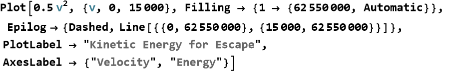
Escape velocity is the speed at which an object’s kinetic energy equals or exceeds the gravitational potential energy binding it to a planet. For a rocket to escape, its total mechanical energy (kinetic plus potential) must be at least zero, meaning it has enough energy to reach infinitely far away without being pulled back. The key inequality compares kinetic energy, , to the magnitude of gravitational potential energy, , where m is the rocket’s mass, M is the mass of the planet, v is the velocity of the rocket, G is the Newtonian gravitational constant, and r is the distance from the center of the planet.

For gravitational escape, the kinetic energy must satisfy the inequality

(9.33)

Since m is on both sides of the inequality, we divide by m,

(9.34)

We isolate v by multiplying through by 2,

(9.35)

We take the square root to establish escape velocity,

(9.36)

The velocity must be at least this value to escape Earth’s gravity.

For Earth, we can use approximate values, , kg, and m. We can now calculate the escape velocity,

(9.37)

We use WL to verify this result.

We can plot this.

Terms and Definitions

Term/Definition 9.34 Escape velocity (symbol ): The minimum speed required for an object to escape a planet's gravitational pull without further propulsion; .

Term/Definition 9.35 Gravitational constant (symbol G): The universal constant in Newton's law of gravitation; .

Term/Definition 9.36 Mass of the planet (symbol M): The mass of the central body (e.g., Earth) exerting gravity.

Term/Definition 9.37 Distance from center (symbol r): The radial distance from the planet's center to the object.

Assumptions (the implicit beliefs the author relies on)

Assumption 9.32: Gravitational escape velocity is derived from energy conservation: kinetic energy must at least equal the magnitude of gravitational potential energy to reach infinity.

Principles

Principle 9.20 Escape velocity: minimum speed where kinetic energy equals gravitational potential energy magnitude:   .

Exercise 9.15: Begin with Term/Definition 9.34 and copy it into your notebook. Reflect on its meaning for a few minutes. Note any thoughts that come to mind. How would you explain this to someone sitting in front of you. Write this down. Then do this for each term/definition, assumption, and principal.

Exercise 9.16:
a) Calculate the escape velocity of a rocket on the Moon, assuming its radius is m and its mass is about kg.
b) Compare the escape velocity of the Earth and of Mars.
c) Assume you are on a plane twice as massive as the Earth but only half the radius, what is its escape velocity?

Problem Solving

Solving problems in mathematics and physics is like embarking on a scientific expedition—you need a clear plan, the right tools, and a sense of curiosity. Whether calculating a rocket’s escape velocity or determining a spring’s safe displacement from equilibrium, a general problem-solving strategy helps you navigate challenges with confidence. This section outlines a step-by-step approach to tackle mathematical problems and their application to physics, empowering you to explore the universe through equations and inequalities.

A systematic method ensures clarity and accuracy when solving problems. Here’s a versatile strategy, adaptable to both mathematics and physics:

Understand the Problem

Write out what you think the problem is. Read the problem carefully to identify what’s given and what’s asked for. Determine the key quantities involved (e.g., variables, constants) and their relationships. Is this a numerical answer, a range, or a graph? For physics problems, identify the physical context, like motion, energy, or forces.

Translate the Problem into Mathematics (or Computation)

Express the problem as equations, inequalities, or diagrams. Assign variables to unknowns, write down known values, and use physical laws or mathematical rules to form relationships.

Plan a Solution

Choose a method to solve the problem, such as algebraic manipulation, graphing, or computational tools. Decide if you’ll solve analytically (by hand or by computer) or numerically (using software). Consider breaking complicated problems into smaller steps.

Execute Your Plan

Carry out your plan, solving equations or inequalities step-by-step. Use techniques from earlier lessons, like factoring quadratics, solving linear systems, or applying absolute values. Check intermediate steps for errors. As you proceed through your studies, your available tools will increase.

Verify the Answer

Ensure the solution makes sense mathematically and physically. Substitute answers back into the original problem, and confirm that the result aligns with physical reality (e.g., positive speeds for motion).

Interpret the Answer

Explain the solution in context, especially for physics problems. What does the answer mean? For example, does a velocity indicate escape from a planet?

Communicate the Answer

Present results clearly, using graphs or words to convey insights.

Terms and Definitions

Term/Definition 9.38 Problem solving: The systematic process of finding solutions to mathematical or physical questions using a structured approach.

Term/Definition 9.39 Understand the problem: The first step — reading carefully, identifying givens, unknowns, and the goal (numerical answer, range, graph, etc.).

Term/Definition 9.40 Translate into mathematics: Converting a physical or word problem into equations, inequalities, diagrams, or computational setups using variables and known laws.

Term/Definition 9.41 Plan a solution: Choosing methods (algebraic, graphical, computational) and breaking complex problems into smaller steps.

Term/Definition 9.42 Execute the plan: Performing the calculations or manipulations step-by-step using learned techniques (factoring, solving equations, etc.).

Term/Definition 9.43 Verify the answer: Checking the solution mathematically (substitution) and physically (does it make sense?).

Term/Definition 9.44 Interpret the answer: Explaining the solution in physical or real-world context (e.g., what does the velocity mean?).

Term/Definition 9.45 Communicate the answer: Presenting results clearly (equations, graphs, words) for understanding and sharing.

Assumptions (the implicit beliefs the author relies on)

Assumption 9.33: Problem solving in math and physics follows a repeatable, structured strategy applicable to any problem.

Assumption 9.34: Careful reading and clear identification of givens/unknowns are essential for success.

Assumption 9.35: Physical problems can always be translated into mathematical form (equations, inequalities, graphs).

Assumption 9.36: Execution must be step-by-step to catch errors early.

Assumption 9.37: Verification (math + physics) is mandatory — answers can be mathematically correct but physically meaningless.

Assumption 9.38: Interpretation connects math back to reality (physical meaning, units, context).

Principles

Principle 9.21: Adapt strategy to problem type: equations for exact values, inequalities for ranges, graphs for visualization.

Exercise 9.17: Begin with Term/Definition 9.38 and copy it into your notebook. Reflect on its meaning for a few minutes. Note any thoughts that come to mind. How would you explain this to someone sitting in front of you. Write this down. Then do this for each term/definition, assumption, and principal.

Electric Circuits where Voltage or Current must Stay Within Certain Bounds

Electric circuits power our world, from light bulbs to spacecraft systems. To ensure circuits operate safely, voltages and currents must often stay within specific limits, like keeping a resistor’s current below a threshold to avoid overheating. Inequalities help us define these safe ranges, connecting mathematics to practical physics. This section applies the problem-solving strategy to circuits, using your skills to analyze voltage and current constraints and explore the physics of electricity.

Current in a Resistor

A resistor in a circuit has resistance R=5 Ω. To prevent overheating, the current I must be less than 2 A. Using Ohm’s Law V=I R, what are the allowed voltages across the resistor?

Step 1: Understand

The problem asks for voltages V that keep the current I<2 A. Given that R=5 Ω, we need a range of voltages ensuring safe operation.

Step 2:   Translate

Applying Ohm’s Law, we write

(9.38)

Since I<2, we conclude,

(9.39)

So, the voltage must be less than 10 V. Since the direction of the current matters, consider absolute values

(9.40)

So,

(9.41)

This implies -10<V<10

Step 3:   Plan

Solve the inequality -10<V<10. Use the general strategy for inequalities: identify critical points, test regions, and visualize. Since it’s a simple linear inequality, we can also verify directly.

Step 4:   Execute

The inequality -10<V<10 suggests voltages between -10 and 10 volts. Test a point, like V=5 V

(9.42)

For V=15 V

(9.43)

The inequality holds for voltages between -10 and 10. Use Wolfram Language:

This confirms −10<V<10.

Step 5:   Verify

We need to check the boundary points. For V=10 we see that

(9.44)

This is not less than 2. The result makes physical sense since voltages too high drive excessive current, risking damage.

Step 6:   Interpret

The resistor operates safely for voltages between -10 and 10 units, corresponding to currents between -2 and 2 A. This ensures the resistor doesn’t overheat, protecting the circuit. Visualize on a number line:

Here we see the range of safe voltages.

Power in a Circuit

Let’s say that we have a circuit component with resistance R=10 Ω. We must then keep power dissipation below 40 W to avoid failure. What are the allowed currents?

Step 1:   Understand

We need to find the current where P<40 W, given R = 10 Ω.

Step 2:   Translate

Power is given by the expression

(9.45)

We can simplify this to

(9.46)

Step 3:   Plan

We solve the inequality (9.46), then we find the roots, test the intervals, and visualize.

Step 4:   Execute

We convert (9.46) into an equation and solve it.

(9.47)

We test the region less than -2, between -2 and 2, and greater than 2. For I-1

(9.48)

For I=3

(9.49)

The inequality holds for currents between -2 and 2. We can use WL to verify this. Note, we have to change the variable for current to J, since I is the built-in symbol for the imaginary unit.

This confirms that currents must be between -2 and 2.

Step 5:   Verify

At I-2, A, this is not less than 40, so the boundary is excluded.

Step 6:   Interpret

Current beyond ±2 A are excluded, since they will produce excessive heat, that will damage the circuit. We can visualize this,

Terms and Definitions

Term/Definition 9.45 Power (symbol P): The rate of energy dissipation in a circuit; for resistors .

Term/Definition 9.46 Overheating: Excessive power dissipation (P > threshold) causing damage to circuit components.

Term/Definition 9.47 Safe operating range: The bounds on voltage or current where the circuit operates without failure (e.g., I < 2 A, P < 40 W).

Assumptions (the implicit beliefs the author relies on)

Assumption 9.39: Circuits must operate within safe voltage/current/power bounds to prevent overheating or failure.

Principles

Principle 9.22: Add dashed lines (Epilog) to mark thresholds (e.g., power limit, current limit).

Principle 9.23: Physical meaning details solution region = safe operating voltages/currents (no overheating, no damage).

Principle 9.24: Apply general problem-solving strategy: understand → translate → plan → execute → verify → interpret.

Exercise 9.18: Begin with Term/Definition 9.45 and copy it into your notebook. Reflect on its meaning for a few minutes. Note any thoughts that come to mind. How would you explain this to someone sitting in front of you. Write this down. Then do this for each term/definition, assumption, and principal.

Exercise 9.19:
a) A circuit has a resister having R=10Ω. Given a current of I=2 A, calculate the voltage V using Ohm’s law. Assume there is a safe range of voltage between 10 V to 20 V. Verify that the voltage is within this range.
b) For a circuit with a resistor R=5 Ω and a safe voltage range of 5 V to 15 V, determine the range of current I that keeps the circuit safe.
c) A component with resistance R=10  Ω operates with a current I=3 A. Calculate the power dissipated using and check if it stays below the safe limit of 40 W.
d) Given a circuit with R=8  Ω and a power limit of 32 W, use to find the maximum safe current I. Then, calculate the corresponding voltage V and ensure it falls between 10 V and 20 V.
e) For a circuit with R=6  Ω, if the voltage V=12 V, calculate the current I using Ohm’s law and the power . Verify if the power is within a safe limit of 24 W.
f) A circuit has R=4 Ω and operates with a voltage range of 4 V to 12 V. Determine the range of current I and power P using Ohm’s law and . Test if V=10 V keeps the circuit in the safe operating region.

Thermal Equilibrium

Thermal equilibrium occurs when objects in contact reach the same temperature, balancing heat flow in systems like engines, refrigerators, or even a cup of coffee cooling in a room. Inequalities help us define the temperature ranges where systems achieve or maintain equilibrium, ensuring safe or efficient operation. This section applies your inequality-solving skills to thermal equilibrium, connecting mathematics to the fascinating physics of heat and energy transfer.

Safe Operating Temperature

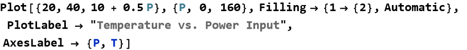
A machine’s component must operate at a temperature T (in degrees Celsius) between 20°C and 80°C to maintain thermal equilibrium with its surroundings and avoid damage. If the component’s temperature is related to power input P by T=10+0.5P, what are the allowed power inputs?

Step 1:   Understand

The problem asks for power inputs P that keep the temperature T between 20°C and 80°C. Given: T=10+0.5P. We need the range of P ensuring safe operation.

Step 2:   Translate

The allowable range of temperature is,

(9.50)

If we substitute T=10+0.5P,

(9.51)

Step 3:   Plan

We must solve the inequality.

Step 4:   Execute

The expression (9.48) is a compound inequality that we must break into two parts,

(9.52)

and

(9.53)

We combine these to get 20<P<140. We can check this using WL:

This confirms our estimate.

Step 5:   Verify

We must now test the boundary points: At P=20, T=10+0.5⋅20=20, this is not  greater than 20 and is excluded. At P=140, T=10+0.5⋅140=80, this is also excluded. We need to pick a point within the other region, so we choose P=50, though any choice between 20 and 140 would be as good, we get

(9.54)

Since this in within the range stated in (9.47), the solution holds.

Step 6:   Interpret

The machine operates safely for power inputs between 20 and 140 W, keeping its temperature between 20°C and 80°C for thermal equilibrium. Power inputs outside this range could overheat or underperform the component. We can visualize this:

Heat Transfer Constraint

Two objects in contact, with temperatures and , approach thermal equilibrium. Suppose is adjusted by a heater’s power P according to the expression

(9.55)

We have somehow determined that equilibrium requires the temperature difference

(9.56)

If we determine that , what are the allowed power inputs?

Step 1:   Understand

We need to find the power P where the temperature difference between and is less than 10°C.

Step 2:   Translate

If we substitute (9.55) into (9.56) we get,

(9.57)

We can apply the definition of an absolute value,

(9.58)

Step 3:   Plan

We must solve the compound inequality.

Step 4:   Execute

We seek to solve (9.58) by adding 10 to each side,

(9.59)

We the divide through by 50,

(9.60)

We can check this using WL:

This confirms our estimate.

Step 5:   Verify

We must now test the boundary points: At P=0.2, , we then put this into (9.58), |310-310|=0<10°C, this is allowed and the solution holds. At P=0.5, , we then put this into (9.53), |325-310|=15>10°C, so this is not allowed.

Step 6:   Interpret

Power inputs between 0 and 0.4 W keep the temperature difference below 10°C, ensuring near-thermal equilibrium. Larger power inputs cause excessive temperature differences, disrupting equilibrium. We can visualize this:

Terms and Definitions

Term/Definition 9.48 Thermal equilibrium: The state where objects in contact reach the same temperature and heat flow stops (no net energy transfer).

Term/Definition 9.49 Temperature (symbol T): A measure of the average kinetic energy of particles in a system; SI unit Kelvin (K); here also used in Celsius (°C) for practical examples.

Term/Definition 9.50 Power input (symbol P): The rate at which energy is supplied to a system (e.g., by a heater); measured in watts (W).

Term/Definition 9.51 Heat flow: The transfer of thermal energy between objects at different temperatures; stops at equilibrium.

Term/Definition 9.52 Temperature difference (symbol Δ T or ): The absolute difference in temperature between two objects; drives heat flow.

Assumptions (the implicit beliefs the author relies on)

Assumption 9.40: Thermal equilibrium occurs when objects in contact have the same temperature (no net heat flow).

Assumption 9.41: Temperature differences drive heat flow; equilibrium requires Δ T ≈ 0 or within safe bounds.

Assumption 9.42: Power input (P) directly affects temperature in a linear way in simple models (e.g., T = 10 + 0.5 P).

Assumption 9.43: Physical systems (machines, components) have safe temperature ranges to avoid damage or inefficiency.

Assumption 9.44: Absolute value correctly measures temperature difference regardless of which is higher.

Principles

Principle 9.25: Thermal equilibrium: systems in contact reach the same temperature; heat flow stops when ΔT = 0.

Principle 9.26: Safe operating temperature: components must stay within bounds (e.g., 20°C < T < 80°C) to avoid damage or inefficiency.

Exercise 9.20: Begin with Term/Definition 9.48 and copy it into your notebook. Reflect on its meaning for a few minutes. Note any thoughts that come to mind. How would you explain this to someone sitting in front of you. Write this down. Then do this for each term/definition, assumption, and principal.

Exercise 9.21:
a) Given a system where the temperature difference and the power input P=30 W, use the expression to verify if thermal equilibrium is achieved. Adjust P if necessary.
b) For a system with a power input P between 20 W and 80 W, determine the allowable range of temperature difference using the expression . Check if C. Verify that the solution is within this range.
c) If the desired temperature difference is 15°C, calculate the required power input P using . Verify the solution and interpret the result.
d) For a system where P=50 W, determine if the temperature difference falls within the allowable range of 20°C to 32°C. Adjust P if it does not meet the condition.
e) For a new system with a modified constant where , calculate the power input P needed to maintain a temperature difference of 25°C. Compare this with the original system.
f) Using the graph of temperature difference vs. power input, estimate the power input P when . Confirm the value using the equation and discuss any discrepancies.

Thermodynamic Systems

Imagine a steaming cup of coffee cooling in a room or a car engine converting fuel into motion—these are examples of thermodynamic systems, where energy, heat, and matter interact to produce change. A thermodynamic system is any defined region we study, like a gas in a container, a liquid in a pipe, or even a star—so long as we track properties like temperature, pressure, or volume.

Thermodynamic systems come in three main types, each characterized by how they interact with their surroundings:

Isolated Systems: These exchange neither energy (like heat) nor matter with their surroundings. Picture a perfectly insulated thermos keeping coffee hot forever. Isolated systems are rare but help us understand energy conservation.

Closed Systems: These exchange energy but not matter. A sealed gas cylinder heated by a flame is a closed system, as heat changes its pressure or temperature, but no gas escapes.

Open Systems: These exchange both energy and matter. A boiling pot of water is an open system, losing steam (matter) and gaining heat from the stove (energy).

Each system has properties like temperature, pressure (the force exerted by particles), and volume (the space it occupies). Inequalities help us define safe or efficient ranges for these properties, ensuring systems like engines or refrigerators operate properly. For now, we’ll use familiar tools—equations and inequalities—to explore simple thermodynamic constraints, setting the stage for deeper discoveries later.

Pressure in a Gas Container

A gas in a closed system (like a sealed container) operates safely when its pressure P is between 1 and 5 units called a pascal and denoted Pa. The pressure is related to temperature T by P=0.01T, assuming constant volume. What are the allowed temperatures?

Step 1:   Understand

The problem asks for temperatures T that keep pressure P between 1 and 5 Pa. Given that P=0.01T. We need the temperature range for safe operation.

Step 2:   Translate

We can define the pressure constraint

(9.61)

We substitute the pressure-temperature relation

(9.62)

Multiplying by 100, we get

(9.63)

Step 3:   Plan

We must solve the compound inequality.

Step 4:   Execute

We choose to test a temperature within the rang defined by (9.63). Let’s choose T=300° C. By the statements in Step 1 we then have,

(9.64)

This definitely falls within the range specified in (9.63), so the solution seems to work.

We can check this using WL:

This confirms our estimate.

Step 5:   Verify

We must now test the boundary points: At T=100° C, P=1 Pa, This is excluded. At T=500° C, P=5 Pa. This is also excluded. So the temperature must be between 100° C  and 500°  C so the pressure is between 1 Pa and 5 Pa, as we have predicted.

Step 6:   Interpret

Physically, temperatures too high could overpressurize the container, while too low could impair function. The system is safe when the temperature is between 100° C and 500° C, keeping the pressure between 1 Pa and 5 Pa. We can visualize this:

Temperature Difference in a Heat Exchanger

An open system, like a heat exchanger, transfers heat between two fluids with temperatures and . We have determined that, for efficient operation, the temperature difference ∣. If , where P is power input, and , what are the allowed power inputs?

Step 1:   Understand

We need to find the power where the temperature difference is less than 20° C.

Step 2:   Translate

We have identified the condition

(9.65)

We substitute the condition

(9.66)

This give us

(9.67)

We can rewrite this,

(9.68)

Step 3:   Plan

We must, again, solve the compound inequality.

Step 4:   Execute

We solve,

(9.69)

Add 15,

(9.70)

Divide by 30,

(9.71)

We can check this using WL:

This confirms our estimate.

Step 5:   Verify

We must now test the boundary points: At P=0.5 Pa, ° C, so the temperature difference is 0° C, which is less than 20° C, as required. At T=1.5° C, ° C, now the temperature  difference is 30° C, which is greater than 20° C, so this is excluded. At P=7/6 Pa, then ° C, the temperature difference here is 20° C = 20° C, this is also excluded Our solution is thus correct.

Step 6:   Interpret

Power inputs between -1/6 Pa and 7/6 Pa units keep the temperature difference in the safe operating range. We can visualize this:

Exercise 9.22:
a) Given a closed system with a constant volume where pressure P and temperature T are related by P=0.01T, calculate the pressure when the temperature is 300 K. Verify if this falls within the safe operating range of 100 Pa to 500 Pa.
b) For a system where P=0.01T and the safe pressure range is 200 Pa to 400 Pa, determine the allowable temperature range. Test if T=250 K is within this range.
c) In a heat exchanger, the temperature difference °C and power input P=15 W. Use the relation to check if the system operates efficiently. Adjust P if necessary.
d) For a thermodynamic system with P=0.01T and a safe temperature range of 100 K to 400 K, calculate the corresponding pressure range. Determine if P=300 Pa is within the safe operating conditions.
e) A system has a pressure-temperature relationship P=0.02T and a heat exchanger where . If 24° C, find the power input P and the corresponding temperature T. Ensure T is between 100 K and 500 K.
f) Using the graph of pressure vs. temperature, estimate the temperature when P=250 Pa. Confirm the value using P=0.01T and discuss any discrepancies within the safe range of 100 Pa to 500 Pa.

Optimization

Optimization is like finding the perfect setting for a spaceship’s engine or the ideal temperature for a chemical reaction—it’s about discovering the best possible value within given bounds. In physics and mathematics, optimization means finding the maximum or minimum of a quantity, like energy, power, or temperature, while respecting constraints like safe operating ranges. This section introduces optimization using the inequalities and equations you’ve learned, reversing the problems we’ve solved to find optimal values.

Maximizing Power in an Electric Circuit

In a previous example, we found that a resistor has a resistance of 5 Ω, this operates safely when the current satisfied |I|<2 A. This leads to voltages |V|<10 V via Ohm’s law (V=I R). So let’s reverse this process to find the maximum power that the resistor can safely dissipate, where .

Step 1:   Understand

The problem asks for the maximum power P within the constraint |I|<2 A. We further know that the resistance R is 5 Ω. We need to find the highest power without exceeding the current limit.

Step 2:   Translate

For our situation, the power is given by,

(9.72)

Step 3:   Plan

Since we have the condition |I|<2 A, and power depends on its square. Assuming this to be 2 A will give us the maximum power. Note that this is a quadratic expression.

Step 4:   Execute

For I=2,

(9.73)

At I=-2, we also have,

(9.74)

So, the maximum power is 20 W.

Step 5:   Verify

We have already tested the boundary points, the answer is not strictly within the limit, but it is the maximum possible.

Step 6:   Interpret

Physically, higher currents would violate the safety constraint. The resistor can safely dissipate up to (but not including) 20 W at currents just below 2 or -2 A.

We can visualize this:

Minimizing Temperature Difference in a Heat Exchanger

In the “Thermodynamic Systems” section, we found that a heat exchanger with and requires a temperature difference |T_1 - T_2| < 20 °C, giving power inputs between -0.167 and 1.167 units. Now, let’s find the power that minimizes the temperature difference .

Step 1:   Understand

The problem asks for the power P that minimizes the temperature difference , subject to -0.167 < P < 1.167. Given that , .

Step 2:   Translate

The temperature difference is,

(9.75)

Step 3:   Plan

Minimize|30P - 15|, or put another way, we need to find the absolute value that is smallest. This occurs when 30P-15=0. We need to solve for this point. Then we need to check to see if this lies within the constraint.

Step 4:   Execute

So, we need to solve,

(9.76)

This gives us,

(9.77)

We can see that -0.167 < 0.5 < 1.167 satisfies this condition.

Step 5:   Verify

We write the WL code

so out solution is correct.

We know test the boundaries: At P=−0.167, , then|35 - 55| = 20, so this is excluded. At P = 1.167, , ∣and|75 - 55| = 20, also excluded.

Step 6:   Interpret

Physically, equal temperatures optimize heat exchanger efficiency. A power input of 0.5 Pa makes , minimizing the temperature difference to 0°C, ideal for thermal equilibrium within the constraint.

We can visualize this:

Terms and Definitions

Term/Definition 9.53 Optimization: The process of finding the maximum or minimum value of a quantity (e.g., power, temperature difference, energy) subject to constraints (e.g., safe operating ranges, bounds).

Term/Definition 9.54 Maximizing: Finding the highest possible value of a quantity within constraints (e.g., maximum safe power dissipation).

Term/Definition 9.55 Minimizing: Finding the lowest possible value of a quantity within constraints (e.g., minimum temperature difference for efficiency).

Term/Definition 9.56 Constraint: A restriction or bound on variables (e.g., |I| < 2 A, < 10°C, P < 40 W).

Term/Definition 9.57 Heat exchanger: A device/system that transfers heat between two fluids (or objects) at different temperatures.

Term/Definition 9.58 Equilibrium (in heat exchanger): The state where temperature difference is minimized or within safe limits for efficient operation.

Assumptions (the implicit beliefs the author relies on)

Assumption 9.45: Power dissipation in resistors () must stay below a damage threshold.

Assumption 9.46: Temperature in simple heater models is linear with power input (T = 10 + 0.5 P).

Assumption 9.47: Heat exchangers operate efficiently when temperature difference is small (e.g., < 10°C).

Principles

Principle 9.27: Optimization finds max/min values under constraints — critical for safe/efficient physical systems (e.g., max power, min temperature difference).

Exercise 9.23: Begin with Term/Definition 9.53 and copy it into your notebook. Reflect on its meaning for a few minutes. Note any thoughts that come to mind. How would you explain this to someone sitting in front of you. Write this down. Then do this for each term/definition, assumption, and principal.

Exercise 9.24:
a) Given a closed system with a constant volume where pressure P and temperature T are related by P=0.01T, calculate the pressure when the temperature is 300 K. Verify if this falls within the safe operating range of 100 Pa to 500 Pa.
b) For a system where P=0.01T and the safe pressure range is 200 Pa to 400 Pa, determine the allowable temperature range. Test if T=250 K is within this range.
c) In a heat exchanger, the temperature difference °C and power input P=15 W. Use the relation to check if the system operates efficiently. Adjust P if necessary.
d) For a thermodynamic system with P=0.01T and a safe temperature range of 100 K to 400 K, calculate the corresponding pressure range. Determine if P=300 Pa is within the safe operating conditions.
e) A system has a pressure-temperature relationship P=0.02T and a heat exchanger where . If 24° C, find the power input P and the corresponding temperature T. Ensure T is between 100 K and 500 K.
f) Using the graph of pressure vs. temperature, estimate the temperature when P=250 Pa. Confirm the value using P=0.01T and discuss any discrepancies within the safe range of 100 Pa to 500 Pa.

Linear Programming

Any method that uses a set of linear constraints that can be used to optimize some important some specific quantity is what we can call linear programming. One illustration of linear programming is planning a space mission to get the most out of limited resources, such as maximizing power output or minimizing energy use while staying within safe limits.

Maximizing Power in an Electric Circuit, Part II

Previously, we found that a resistor with R=5 Ω operates safely when the current that satisfies  the constraint|I| < 2 A, giving voltage constraints|V| < 10 V via Ohm’s Law V=I R. Now, imagine a circuit with two power sources, with voltages and , and we want to maximize the total power delivered, described by the expression, presumably derived elsewhere, , subject to these safety constraints,

(9.78)

(9.79)

Step 1:   Understand

The problem asks us to maximize , representing power, while satisfying the constraints (9.78) and (9.79).

Step 2:   Translate

The expression we need to maximize is,

(9.80)

The constraint inequalities define the region in our coordinate plane where and are valid.

Step 3:   Plan

Plot the constraints to find the feasible region (from Linear Inequalities on a Coordinate Plane above). The maximum value of (9.78) occurs at a corner of this region. Find the corners by solving the constraint equations where they intersect, evaluate the expression at each corner, and use Wolfram Language to visualize.

Step 4:   Execute

Draw the constraints. We convert (9.78) into an equation,

(9.81)

and this forms a diagonal line from (10,0) to (0,10). gives us the axis, and gives us the axis.

We now evaluate (9.78) at each corner. At (0,0) we are multiplying all of the factors by zero, so we are left with 0. At (10,0) we have 20, and at (0,10) we have 30. So the largest power is 30 units when and .

Step 5:   Verify

Check (0, 10): 0+10≤10, 0≥0, and 10≥0. Next we test an interior point, e.g., (5, 5):

(9.82)

Step 6:   Interpret

Physically, by (9.78),   contributes more of the power, so maximizing it is logical. By so setting the voltages we are optimizing the circuit’s performance within safety limits.

Minimizing Temperature Difference in a Heat Exchanger, part II

Previously, we had a heat exchanger with , , with , giving power P between -0.167 and 1.167 units. Now, suppose two power inputs and affect , and we want to minimize the temperature difference , subject to the constraints:

(9.83)

(9.84)

Step 1:   Understand

Maximize , subject to the constraints (9.83) and (9.84). Find the power outputs making closest to 55°C.

Step 2:   Translate

We must maximize

(9.85)

subject to the constraints defined in (9.83) and (9.84).

Step 3:   Plan

Minimize by setting , then check if it’s in a feasible region. If not, then evaluate it at the corners.

Step 4:   Execute

So, we need to solve,

(9.86)

So,

(9.87)

We test this according to (9.83), substituting (9.87) for ,

(9.88)

Multiply by 2,

(9.89)

Subtract by 1.5,

(9.90)

This is outside the constraint (9.83). We now draw the regions.

We have points at (0,0),(2,0), and (0,2). If we test these by applying the values to (9.84) we get, respectively 15°C, 5°C,and 25°C. The smallest difference is 5°C at units and units.

Step 5:   Verify

The point (2,0) satisfies our constraints, 2+0=2≤2, 2>=0, and 0>=0.   We can also test another point, say (1,1), this gives us, by (9.84) 15°C>5°C.

Step 6:   Interpret

We have seen that prioritizing reduces the temperature gap and optimizes the heat exchanger’s efficiency.

Terms and Definitions

Term/Definition 9.59 Linear programming: A mathematical method to optimize (maximize or minimize) a linear objective function subject to a set of linear constraints (inequalities and/or equations).

Term/Definition 9.60 Objective function: The linear expression to be maximized or minimized (e.g., power ).

Term/Definition 9.61 Constraint: A linear inequality or equation restricting the feasible values of variables (e.g., ).

Term/Definition 9.62 Feasible region: The collection of all points (combinations of variables) that satisfy all constraints; typically a polygon in the coordinate plane.

Term/Definition 9.63 Corner point (or vertex of feasible region): The intersection points of the constraint boundaries; in linear programming, optimal values occur at one or more corner points.

Assumptions (the implicit beliefs the author relies on)

Assumption 9.48: Linear programming applies to problems with a linear objective and linear constraints (e.g., maximizing power, minimizing temperature difference).

Assumption 9.49: Optimal solutions in linear programming occur at corner points (vertices) of the feasible region.

Assumption 9.50: Testing corner points and interior points verifies the optimum.

Principles

Principle 9.28: General strategy: Understand → Translate (objective + constraints) → Plan (plot feasible region) → Execute (evaluate at corners) → Verify → Interpret.

Exercise 9.25: Begin with Term/Definition 9.59 and copy it into your notebook. Reflect on its meaning for a few minutes. Note any thoughts that come to mind. How would you explain this to someone sitting in front of you. Write this down. Then do this for each term/definition, assumption, and principal.

Exercise 9.26:
a) For an electric circuit with constraints ∣V, and an objective function to maximize power, determine the optimal values of
and within the feasible region. Verify the maximum power.
b) Given a circuit with constraints V, V, and V, and the quantity we are optimizing is , find the values of
and that maximize power. Check the solution against the constraints.
c) In a heat exchanger with constraints °C, T2≤60°C, and 10°C, and the quantity we are optimizing is (where P is power input), minimize the temperature difference. Assume P≤10 W and find the optimal , , and P.
d) For a circuit with constraints V, 0 V, and V, and the quantity we are optimizing is , determine the maximum power. Test the boundary points to confirm the solution.
e) Given a heat exchanger with constraints 5°C, °C, °C, and P≤8 W, minimize the temperature difference . Find the optimal values of , , and P.
f) For a system combining a circuit (V, V, V, maximize ) and a heat exchanger (, °C, °C, P≤12 W), solve for the optimal , , , , and P within their respective feasible regions.

Summary

Write a summary of this lesson.

For Further Study

Navy Education and Training Professional Development and Technology Center, (1980) Mathematics, Basic Math and Algebra, NAVEDTRA 144139, Reprinted in 1985 (available for free at the Internet Archive https://archive.org/details/US_Navy_Training_Course_-_Mathematics_Basic_Math_and_Algebra). This is the first of a comprehensive set of manuals for training sailors in basic math.

Ray Steege, Kerry Bailey, (2018), Intermediate Algebra, McGraw-Hill, Schaum’s Outline Series. This book has many chapter relating to inequalities, and it has lots of solved problems to test your abilities.