Lesson 8: Symbolic Computation and Higher-Order Equations

Introduction

Welcome to Lesson 8, where we embark on an exciting journey into symbolic computation—a skill that transforms complex mathematics into something you can conquer with the Wolfram Language. In Lesson 5, you got your feet wet with this powerful tool, learning how to compute and explore. Lesson 6 introduced you to linear equations of the form a x + b = 0, showing how to solve for straight-line solutions with ease. Then, in Lesson 7, we stepped up to quadratic equations of the form , mastering techniques like factoring and the quadratic formula, all while using WL to visualize parabolas and their roots. Now, it’s time to climb higher; in this lesson we’re tackling polynomial equations, specifically cubic equations of the form , and quartic equations of the form .

Why should you care? Polynomials are the building blocks of representation of many physical phenomena. The trajectory of a rocket, the bending of a beam, or the oscillations in an electric circuit often involve terms like or . Unlike the straight lines of Lesson 6 or the gentle curves of Lesson 7, these higher-degree equations can twist and turn in surprising ways, and solving them by hand gets tricky fast. That’s where symbolic computation shines. With the Wolfram Language, you’ll solve cubics and quartics—finding all their roots, real or complex—and plot them to see how their shapes reflect their behavior.

This lesson starts with a review of some methods we have already seen along with some new ones. Then we will introduce the idea of something called a workflow. Some more commands in WL will be introduced to make life easier. We will then turn to finding the roots of polynomial equations. Then we learn of a WL function to find the discriminant. Next, we’ll dive into cubic equations, using commands like Solve[] to reveal up to three roots and plotting them to uncover their behavior. We will then dive into electric circuits as a physical example. Then we’ll conquer quartic equations, which can have up to four roots, and see how Wolfram handles their complexity with precision. We then go to higher-degree equations. Then we will explore how to manipulate polynomials. Along the way, you’ll discover how symbolic computation bridges the gap between algebra and intuition, a skill that’s invaluable for the physics challenges ahead.

Basics of Symbolic Computation in WL

Symbolic computation is like having a super-smart math assistant who can manipulate equations, simplify expressions, and solve problems without needing every number spelled out upfront. Unlike numerical computation (e.g., calculating 2 + 3 = 5), symbolic computation works with symbols—letters like x, a, or b—to find general solutions or rewrite expressions in useful forms. In physics, this is a game-changer: it lets us derive formulas, explore relationships, and solve equations that describe everything from falling objects to orbiting planets. The Wolfram Language (WL) makes this accessible, and in this section, we’ll master its basic tools to set the stage for polynomials, cubics, and quartics.

You’ve already used some symbolic power. In Lesson 5, you played with expressions and ran simple commands. Lesson 6 had you solving linear equations like 2x + 3 = 0, and Lesson 7 we used Solve[] for quadratics like , even handling complex roots. Now, we’ll broaden those skills with key WL functions: Simplify[], Expand[], Factor[], and Solve[]. These will help us manipulate and solve higher-degree equations effortlessly.

Physics often gives us messy equations that need tidying up. The Simplify[] function takes a complicated expression and makes it as concise as possible.

WL recognizes that cancels out. This is handy when deriving formulas.

Sometimes, you need to see all the terms laid out, especially when working with polynomials. The Expand[] function does just that.

This matches what you’d get by applying the FOIL method (First, Outer, Inner, Last) from algebra, but WL does it instantly.

Factoring breaks polynomials into simpler pieces, a skill you used in Lesson 7 to solve quadratics.

This is the reverse of expanding. This is crucial for solving equations—finding where means setting each factor to zero (x = -2 or x = 3). Later, we’ll factor cubics and quartics to uncover their roots.

The Solve[] function is your go-to for finding roots, and it shines with symbolic computation. You’ve used it before.

Let’s combine these tools. Suppose you’re given . First, you simplify it.

You get ( 1 ).

Now, if this were an equation set to zero , it simplifies to 1 = 0, which has no solution—a clue about consistency in physical models. Try plotting it.

The graph is a flat line at y = 1, never crossing zero, confirming no roots.

These basics—simplifying, expanding, factoring, and solving—are your toolkit for symbolic computation. As we move to polynomials, cubics, and quartics, you’ll use them to tame higher-degree equations, revealing their roots and shapes with WL’s help. Practice these commands, and you’ll be ready to explore the wild curves of cubics and quartics next!

Terms and Definitions

Term/Definition 8.1 Expand[] (Wolfram Language function): A command that expands an expression, distributing terms and showing all individual components (reverse of factoring).

Term/Definition 8.2 Factor[] (Wolfram Language function): A command that factors a polynomial into simpler factors or irreducibles.

Term/Definition 8.3 Expression (in WL): The fundamental data type in Wolfram Language; everything (numbers, variables, equations, plots, text, etc.) is an expression.

Term/Definition 8.4 Token: The basic building blocks of an expression (symbols like x, y, operators like +, functions like Plus[]).

Assumptions (the implicit beliefs the author relies on)

Assumption 8.1: Beginners can quickly use symbolic commands (Simplify, Expand, Factor, Solve) with minimal prior coding experience.

Assumption 8.2: Verification of symbolic results (e.g., substitution, expansion, plotting) remains necessary.

Principles

Principle 8.1: Use Simplify[] to reduce expressions to their cleanest form.

Principle 8.2: Use Expand[] to distribute and reveal all terms (useful for verification and understanding).

Principle 8.3: Use Factor[] to break polynomials into simpler factors (reverse of Expand[]; key for solving equations).

Principle 8.4: Use Solve[equation, variable] to find exact symbolic solutions (roots, general forms).

Principle 8.5: Combine commands: Simplify first, then Factor or Expand, then Solve for maximum insight.

Exercise 8.1: Begin with Term/Definition 8.1 and copy it into your notebook. Reflect on its meaning for a few minutes. Note any thoughts that come to mind. How would you explain this to someone sitting in front of you. Write this down. Then do this for each term/definition, assumption, and principal.

Exercise 8.2:
a) Simplify, .
b) Expand (x+2)(x-3).
c) Factor .
d) Plot

Workflows

Symbolic computation in the Wolfram Language (WL) isn’t just about individual tools—it’s about stringing them together into a combination that gets you from a raw equation to a useful answer. Think of this as a recipe where each tool is an ingredient, and the workflow is how you mix them to cook up a solution.

A workflow is a sequence of WL commands tailored to your goal—whether it’s simplifying an expression, finding roots, or preparing for visualization. In Lesson 7, you might have factored to (x - 2)(x + 2) = 0  and solved it. That’s a mini-workflow: factor, then solve. Here, we’ll build on that, using multiple tools to handle trickier expressions, setting the stage for higher-degree polynomials.

Workflow 1: Simplifying and Solving

Suppose you’re given an expression, . Your goal is to simplify it and check if it equals zero at some point.

Step 1: Simplify it.

Much cleaner!

Step 2: Set it to zero and solve it.

Step 3: Visualize.

This result clearly confirms the root at 0. This workflow—simplify, solve, plot—turns a messy start into a clear result, like finding when an object returns to its starting point.

Workflow 2: Expanding and Factoring

Now try an expression like . You want its simplest polynomial form and roots.

Step 1: Expand it.

This yields a quadratic equation in t.

Step 2: Factor it (if possible)/

Here, it stays in its quadratic form.

Step 3: Solve.

This is an exact rational  number, we can get the numerical approximation by applying N to the end.

Step 3: Plot it.

If you mouse over the curve in MMA its values at that point will appear, you can see where the roots are located. The parabola crosses the x-axis near those roots. This workflow—expand, attempt to factor, solve, plot—helps you see when speed hits zero.

Workflow 2: Building Your Own Workflow

Define your goal: Simplify? Solve? Visualize?
Pick tools: Use Expand[] or ExpandAll[] to unpack, Simplify[] to reduce, Factor[] to break down.
Iterate: Check each step with a plot or Solve[].

Terms and Definitions

Term/Definition 8.5 Workflow (in WL context): A tailored sequence of Wolfram Language commands to achieve a goal (e.g., simplifying an expression, solving an equation, or preparing visualization).

Assumptions (the implicit beliefs the author relies on)

Assumption 8.3: Users can chain commands (e.g., Simplify → Factor → Solve → Plot) to build powerful workflows.

Principles

Principle 8.6: Workflows turn raw expressions into clear results (e.g., messy start → simplified/solved/plotted).

Exercise 8.3: Begin with Term/Definition 8.5 and copy it into your notebook. Reflect on its meaning for a few minutes. Note any thoughts that come to mind. How would you explain this to someone sitting in front of you. Write this down. Then do this for each term/definition, assumption, and principal.

Together[], Apart[]

When you’re dealing with fractions, Together[] combines them into one fraction with a common denominator.

The flip side of Together[], Apart[] breaks a single fraction into sum of simpler fractions; these are called partial fractions.

Terms and Definitions

Term/Definition 8.6 Together[] (Wolfram Language function): A command that combines a sum of fractions into a single fraction with a common denominator.

Term/Definition 8.7 Apart[] (Wolfram Language function): A command that decomposes a single rational expression (fraction of polynomials) into a sum of simpler partial fractions.

Term/Definition 8.8 Partial fractions: The process or result of breaking a rational expression into a sum of simpler fractions (the output of Apart[]).

Term/Definition 8.9 Common denominator: A single denominator shared by multiple fractions after combining them (produced by Together[]).

Assumptions (the implicit beliefs the author relies on)

Assumption 8.4: Partial fraction decomposition is always possible for proper rational expressions (degree of numerator < degree of denominator).

Assumption 8.5: WL commands Together[] and Apart[] are intuitive extensions of manual fraction manipulation.

Principles

Principle 8.7: WL automates fraction manipulation: Together[] for consolidation, Apart[] for breakdown.

Principle 8.8: These tools extend arithmetic fraction rules to polynomials and rational functions.

Exercise 8.4: Begin with Term/Definition 8.6 and copy it into your notebook. Reflect on its meaning for a few minutes. Note any thoughts that come to mind. How would you explain this to someone sitting in front of you. Write this down. Then do this for each term/definition, assumption, and principal.

Exercise 8.5
a) Combine .
b) If we have a potential energy expression, . Interpret the result.
c) Decompose into partial fractions.
d) Combine and then plot the result over t from -2 to 2.

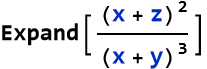
ExpandAll[]

In the Wolfram Language, symbolic computation often means peeling back the layers of an expression to see what’s inside. You’ve already met Expand[] in our toolkit, a command that multiplies out products like (x + 1)(x + 2)  into. But what if your expression is more tangled—nested with fractions, powers, or denominators? That’s where ExpandAll[] comes in. This function goes deeper than Expand[], relentlessly expanding every part of an expression, no matter where it’s hiding. It’s like unpacking a set of Russian Matryoshka dolls—every layer gets opened up. In this section, we’ll explore ExpandAll[].

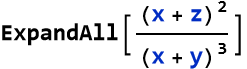
While Expand[] focuses on multiplying out products at the top level, ExpandAll[] digs into every nook and cranny—numerators, denominators, exponents, you name it. It’s especially useful when you’re dealing with rational expressions (fractions) or complex polynomials that need a full breakdown. Let’s start with a simple comparison.

Now try this.

You get the same result here because there’s nothing deeper to expand. But watch what happens when fractions enter the picture.

Where

In older versions of WL Expand was not as good as it is now.

Terms and Definitions

Term/Definition 8.10 ExpandAll[] (Wolfram Language function): A command that fully expands every part of an expression, including nested products, fractions, denominators, exponents, and any hidden multiplications — more thorough than Expand[].

Term/Definition 8.11 Rational expression (in context): A fraction where numerator and/or denominator are polynomials or expressions.

Term/Definition 8.12 Nested expression: An expression inside another expression (e.g., inside denominators, exponents, or parentheses).

Assumptions (the implicit beliefs the author relies on)

Assumption 8.6: Expand[] is sufficient for simple top-level expansion, but ExpandAll[] is needed when expansions are hidden (e.g., in denominators or fractions).

Assumption 8.7: ExpandAll[] will expand every possible multiplication, even deep inside fractions or powers.

Principles

Principle 8.9: Always compare Expand[] vs. ExpandAll[] to see the difference in depth (e.g., fractions stay combined with Expand[], fully expand with ExpandAll[]).

Exercise 8.6: Begin with Term/Definition 8.10 and copy it into your notebook. Reflect on its meaning for a few minutes. Note any thoughts that come to mind. How would you explain this to someone sitting in front of you. Write this down. Then do this for each term/definition, assumption, and principal.

Exercise 8.7
a) Expand .
b) Expand, , then interpret the result.
c) Expand .
d) Expand and then plot the result over t from -2 to 2.
e) Expand , then plot the result over t from 0 to 3.

Roots of Polynomials

The roots of a polynomial are the values of a variable that make the polynomial equal zero—the “solutions” where its graph kisses or crosses the horizontal-axis. In Lesson 6, you found the root of a linear equation like 2x - 4 = 0 was x = 2. Lesson 7 upped the game with quadratics like , giving two roots x = 2, -2. Now, as we explore polynomials in general—expressions like —we’ll see how their degree (the highest power of x) determines the number of roots, and how the Wolfram Language finds them effortlessly. In this section, we’ll use WL tools like Solve[], Roots[], and Factor[] to hunt down roots, visualize them, and get ready for cubics and quartic next.

If we write a general polynomial in the variable x as P(x), its roots are where P(x) = 0. The Fundamental Theorem of Algebra says a polynomial of degree n has exactly n roots, counting repeats and complex numbers. A linear polynomial (degree 1) has 1 root, a quadratic (degree 2) has 2, a cubic (degree 3) has 3, and so on. Some roots are real (visible on a graph), others complex (hidden from the real axis). Let’s start simple and build up.

The Solve[] function is your go-to for roots. Take a quadratic.

Plot it.

Factoring often shows roots directly.

Set each factor to zero and solve for x. In our case x=3 and 2. The same roots as Solve[] gave us. Not all polynomials factor so neatly, but when they do, it’s a shortcut.

The Roots[] function offers another view, especially for exact forms.

Wait, what does || mean? In WL || is another way or writing the word or, just like && is another way of writing and. So this tells us the roots are either 2 or 3, the same result we got before. It’s similar to Solve[] but can be more readable for polynomials.

Use Roots[] when you want a compact root list, though Solve[] is more versatile.

Terms and Definitions

Term/Definition 8.13 Roots (of a polynomial): The values of the variable that make the polynomial equal zero (solutions); where the graph crosses or touches the horizontal axis.

Term/Definition 8.14 Roots[] (Wolfram Language function): Returns a compact list of roots of a polynomial (often more readable than Solve[] for polynomials).

Term/Definition 8.15 || (in WL output): Logical OR; used in Roots[] output to indicate alternative solutions (e.g., x = 2 || x = 3).

Term/Definition 8.16 && (in WL): Logical AND (mentioned in passing as comparison to ||).

Assumptions (the implicit beliefs the author relies on)

Assumption 8.8: Roots[] provides a more compact/readable output for polynomials than Solve[].

Assumption 8.9: Plotting a polynomial visually confirms roots (crossings/touches) and behavior (e.g., parabola shape).

Principles

Principle 8.10: Roots are where a polynomial equals zero—solutions to P(x) = 0.

Principle 8.11 Fundamental Theorem of Algebra: degree n → exactly n roots (real or complex, counting multiplicity).

Exercise 8.8: Begin with Term/Definition 8.13 and copy it into your notebook. Reflect on its meaning for a few minutes. Note any thoughts that come to mind. How would you explain this to someone sitting in front of you. Write this down. Then do this for each term/definition, assumption, and principal.

Exercise 8.9
a) Find the roots of .
b) Factor and then determine the associated roots.
c) Find the roots of .
d) Find the roots of , and then plot it.

The Discriminant

The discriminant is like a crystal ball for polynomials—it tells you how many real roots you’ll find without solving the equation outright. In Lesson 7, you tackled quadratic equations and saw that their roots depend on the quantity . That’s the discriminant for a quadratic, and it’s a game-changer. A positive value means two real roots, zero means one, and negative means none (just complex roots). In general we write a quadratic,

This has the discriminant given here:

We can see where this comes from:

If we assign the upper-case Greek letter delta, Δ, we can define the discriminant

(8.1)

For quadratics this tells us everything! If Δ > 0, there are two distinct real roots. If Δ = 0, there is only one real root (a double root). If Δ < 0, then there are no real roots (only complex conjugates).
Let’s test it. Take

Since this is greater than 0, there are two real roots. We can test this.

We can visualize this:

Now try,

This predicts a single, double, root.

We can visualize this.

This uses the Row command to present the specific label we want.

Then we can try,

This predicts no real roots.

The plot tells the story.

Wait a second, this makes it look like the parabola touches the origin. Looking at it carefully tells us that this is not so. We can redraw this with a subcommand telling where the origin will be.

We see that there is no real solution.

The discriminant is your shortcut to understanding a polynomial’s roots without solving fully—crucial when tweaking physics models (e.g., adjusting initial velocity). Use Discriminant[] to peek ahead, then Solve[] and Plot[] to confirm. As we dive into cubics and quartics, this tool will guide us through their wilder root patterns, linking math to physical events like oscillations or equilibrium points.

Terms and Definitions

Term/Definition 8.17 Discriminant (symbol D and/or Δ): The quantity in a quadratic equation ; determines the nature and number of real roots.

Assumptions (the implicit beliefs the author relies on)

Assumption 8.10: Wolfram Language functions Solve[], Discriminant[], and Plot[] reliably compute and visualize roots and behavior.

Exercise 8.10: Begin with Term/Definition 8.17 and copy it into your notebook. Reflect on its meaning for a few minutes. Note any thoughts that come to mind. How would you explain this to someone sitting in front of you. Write this down. Then do this for each term/definition, and assumption.

Exercise 8.11
a) Find the discriminant of , and then find its roots.
b) Determine the number of roots of and then find the roots.

Cubic Equations

Polynomial equations having the general form,

(8.2)

is what we call a cubic equation. Such equations take us beyond the parabolas of Lesson 7 into a world of twists and turns. With degree 3, cubics can have up to three roots, reflecting more complicated behaviors. Cubics challenge us with three roots—real, repeated, or complex—and the Wolfram Language (WL) makes solving them a breeze. Here, we’ll use Solve[], Factor[], and Discriminant[] to find roots, visualize them, and connect to physical insights.

A cubic’s three roots come, again, from the Fundamental Theorem of Algebra, but their nature varies. The graph might cross the horizontal-axis three times (three real roots), once (one real, two complex), or somewhere in between (e.g., a double root). Unlike quadratics, cubics don’t have a simple formula for hand-solving, but WL’s symbolic power handles them effortlessly.

Like quadratics, unless we have something simple then we must examine the discriminant, Δ. If this is positive, then there are three real roots, if this is zero then there is at least one double root. If it is negative then there is one real and two complex roots.

Let’s start with an example having a factored cubic.

We first look to the discriminant.

This predicts three real roots.

We can then visualize this.

Note that there are three crossings at 1, 2, and 3—a classic cubic shape with a dip and rise.

Now try

This predicts one real and two complex roots.

What the heck is that output? This is called (in WL) a root number. numbers are formatted as where approx is a numerical approximation. As expected we see one real root and two complex roots.

We can visualize this.

We see only one intersection with the horizontal axis, as expected.

Next we try this.

This predicts at least one repeated root.

We can then solve this.

As predicted we have a single repeated root.

We can visualize this.

Imagine a the position of an object on the end of a spring given by,

(8.3)

We want to find the points of equilibrium (where p(t)=0). To do this we use the, now familiar, work flow.

This predicts repeated roots.

We see that there are two repeated roots. We then visualize this to understand the solution.

We can see that there are crossings at 1 (touching) and 2—these are equilibrium points where the system balances

Terms and Definitions

Term/Definition 8.18 Cubic equation: A polynomial equation of degree 3 in the general form .

Term/Definition 8.19 Roots (of a cubic): The values of x that satisfy the equation (solutions); where the graph crosses or touches the x-axis; a cubic has exactly three roots (counting multiplicity), some real, some complex.

Term/Definition 8.20 Discriminant (of cubic): A quantity (computed by Discriminant[] in WL) that predicts the nature of roots (three real, one real + two complex, or repeated roots).

Assumptions (the implicit beliefs the author relies on)

Assumption 8.11: Every cubic equation has exactly three roots (real or complex), counting multiplicity (by the Fundamental Theorem of Algebra).

Assumption 8.12: The discriminant accurately predicts the number and nature of real roots for cubics.

Assumption 8.13: Real roots appear as x-intercepts; complex roots do not cross the real axis.

Assumption 8.14: Cubics always have at least one real root (odd degree polynomials cross the x-axis at least once).

Assumption 8.15: Repeated roots cause touching or inflection at x-axis (multiplicity > 1).

Exercise 8.12: Begin with Term/Definition 8.18 and copy it into your notebook. Reflect on its meaning for a few minutes. Note any thoughts that come to mind. How would you explain this to someone sitting in front of you. Write this down. Then do this for each term/definition, and assumption.

Exercise 8.13
a) Find the discriminant of , and then find its roots.
b) Determine the number of roots of and then plot it.

Electric Circuits

At this stage in our understanding, electric circuits bring physics to life. They are important in everything from flashlights to spacecraft, and you’ve already got the basics down. In Lessons 4 and 6, you explored Ohm’s Law (V = I R), solving linear equations like V - 3I = 0 for simple resistor circuits. Here, we’ll start with series circuits involving resistors, capacitors, and diodes, then dive into a cubic example, showing how symbolic computation uncovers key circuit behaviors.

In a series circuit, components line up one after another—current flows through each in turn. You know from Lesson 4 that resistors in series add up. We get a total resistance

(8.4)

and Ohm’s Law gives the voltage,

(8.5)

For two resistors, say and , at I=1 Amp, then V = 1 Amp × (2 Ω + 3 Ω) = 5 Volts.

So we know how to deal with resistors. We now examine an important circuit device that was originally made from two metal plates separated by an insulator (a material that limits the passage of electricity)—this is called a capacitor. In a resistor the current flows right through, though the resistor reduces the amount of current. In a capacitor the quantity of electricity (a thing that we call charge,—denoted by the symbol Q—this is the electrical version of mass) gets stored in the device so long as a voltage is applied to it. In series, a capacitor’s voltage builds as it charges,

(8.6)

So we are ready to move on. What? Oh, what is C? It is a property of the device that allows charge to be stored, we call it the capacitance of the device. We will not define it exactly here, it requires integral calculus to do that. The capacitance is measured in Farads, where one Farad is one Coulomb per Volt. For now we can think of it as a constant property of the capacitor, measured in Farads. Total voltage might then be written,

(8.7)

For a case with = 2 Ω, C = 1 Farad, I = 1 Amp, at t = 1 second, then  we have,

(8.8)

There are nonlinear devices that we can add to a circuit. One example is a device that allows current to flow in only one direction, a diode. Their voltage-current relation can approximated as

(8.9)

where n is model-dependent, but is 3 in some models. The symbol k here represents a number that we call a scale factor, it makes sure that a certain amount of current flows in the correct direction for a voltage raised to a given power. In series with a resistor, total voltage splits,

(8.10)

Ohm’s Law is perfect for resistors, but diodes bend the rules. Suppose we have a diode in series with a resistor, the current is given by,

(8.11)

If I = 0 Amps, then we have a condition called an open circuit. If we put this value in for (8.11), then we can study the equilibrium of the diode as a cubic equation.

This tells us that we have three possible voltages.

We can see the crossings at -1.88, 0.35, 1.53—these are stable points where current drops to zero.

Now we will look at a series circuit with a resistor (2 Ω), capacitor (1 Farad), and a diode (described by ). Total voltage at t = 0 might balance when I = 0 Amps, this gives us,

(8.12)

We can use WL to solve this problem.

We can add capacitor and resistor effects later, but for I = 1 Amp we can write the voltage,

(8.13)

If we set an expression for the current,

(8.14)

and,

(8.15)

We can then  visualize this.

We see the three equilibrium voltages for the diode.

Workflow for Circuits

Combine Ohm’s law, capacitor charge, and diode nonlinearity.
Solve with Solve[] to find voltages or currents.
Use Discriminant[] to verify root types.
Plot to visualize beyond Ohm’s linearity.

Terms and Definitions

Term/Definition 8.21 Charge (symbol Q): The fundamental quantity of electricity; can be positive or negative; SI unit Coulomb (C).

Term/Definition 8.22 Coulomb (C): SI unit of charge; named after Charles-Augustin de Coulomb (1736–1806).

Term/Definition 8.23 Ampere (A): SI unit of current; 1 A = 1 C/s; named after André-Marie Ampère (1775–1836).

Term/Definition 8.24 Volt (V): SI unit of voltage; 1 V = 1 J/C.

Term/Definition 8.25 Capacitor: A device that stores charge; voltage across it is .

Term/Definition 8.26 Capacitance (symbol C): Property of a capacitor; ability to store charge per volt; SI unit Farad (F).

Term/Definition 8.27 Diode: A nonlinear device allowing current in one direction; approximated by (n often 3 in models).

Assumptions (the implicit beliefs the author relies on)

Assumption 8.16: Units in SI are consistent and interlinked (e.g., A = C/s, V = J/C, Ω = V/A).

Assumption 8.17: Equilibrium in circuits (steady state) occurs when current or voltage stabilizes (e.g., I = 0).

Assumption 8.18: Nonlinear devices (diodes) lead to polynomial/cubic equations for steady-state analysis.

Assumption 8.19: Series components add resistances; total voltage splits across them.

Principles

Principle 8.11: Capacitors store charge; ; in series, voltage adds.

Principle 8.12: Use symbolic solving (Solve[]) to find equilibrium points in nonlinear circuits.

Principle 8.13: Plot current vs. voltage to visualize diode behavior and equilibrium crossings.

Exercise 8.14: Begin with Term/Definition 8.21 and copy it into your notebook. Reflect on its meaning for a few minutes. Note any thoughts that come to mind. How would you explain this to someone sitting in front of you. Write this down. Then do this for each term/definition, assumption, and principle.

Exercise 8.15
a) Solve V=I 100, for current given V=2 V, then plot I vs V . Interpret this result.
b) Compute the discriminant of , then find . Interpret this result.
c) Solve for current then plot the result. Interpret this result.
d) Plot over from -1 to 2. Find the equilibrium points.
e) Solve for current where V=1V, C = 0.1F, and Q=0.2C. Then plot it.

Quartic Equations

Polynomial equations of the general form,

(8.16)

are called quartic equations. These things take us one step higher than the cubics of the previous section, offering up to four roots and even wilder curves. With degree 4, quartics can twist through the horizontal-axis four times, reflecting complicated physical systems. Here, we’ll use Solve[], Factor[], and Discriminant[] to uncover roots, visualize them, and tie them to physics.

A quartic’s four roots (per the Fundamental Theorem of Algebra) can include real roots (where the graph crosses or touches the horizontal-axis) and complex ones (invisible on a real plot). The graph’s shape—often a “W” or multiple humps—depends on its coefficients. Let’s start with a factored quartic.

Note that we have a triple root at x=2.

We can see this if we use Factor[].

This confirms the triple root at 2 and the single roots at -1. We can then plot it.

We see the crossings at -1 and 2—three visible interactions due to the triple root flattening the curve there.

The quartic discriminant is a beast (a polynomial in a, b, c, d, e ), but it predicts root behavior:

Positive: Four real roots or none (depending on other factors).
Zero: Repeated roots.
Negative: Two real, two complex (or other mixes).

For our example above, we have.

Let’s try another.

We expect four real roots, or none.

In this case, there are no real roots.

We can plot this.

We see there are no crossings—the curve stays above the horizontal-axis, as expected.

Let’s try a different case.

This predicts two real roots and two complex roots.

This is what was predicted. We can visualize this.

We see two crossings—real roots show, complex ones don’t.

Imagine a spring-mass system with a quartic potential energy term,

(8.17)

We want to find the positions resulting in equilibrium (places where V(x)=0).

Again we predict two real roots and two complex.

As we predicted. The energy diagram for this looks like this.

We see two crossings—equilibrium positions where energy balances, like stable or unstable points in a complex spring setup.

Workflow for Quartics

Check Discriminant[] to predict real vs. complex.

Use Solve[] for all roots.

Plot to spot real roots visually.

Terms and Definitions

Term/Definition 8.28 Quartic equation: A polynomial equation of degree 4 in the general form .

Term/Definition 8.29 Roots (of a quartic): The values of x that satisfy the equation; a quartic has exactly four roots (real or complex), counting multiplicity.

Term/Definition 8.30 Parabola-like behavior (in quartics): The graph may resemble a W-shape or multiple humps, with up to three turning points.

Assumptions (the implicit beliefs the author relies on)

Assumption 8.20: The discriminant for quartics predicts root behavior (four real, two real + two complex, repeated roots).

Assumption 8.21: Quartics often have at least two real roots (due to even degree), but can have zero, two, or four.

Assumption 8.22: Repeated roots cause touching or flattening at the x-axis (multiplicity > 1).

Principles

Principle 8.14: Use Discriminant[] to preview root behavior before full solving.

Principle 8.15: Use Solve[equation, variable] to find exact roots (real or complex).

Principle 8.16: Use Plot[] to visualize: crossings = real roots; touches = repeated roots; no crossing = complex roots.

Principle 8.17: Combine discriminant, solving (Solve[]), and plotting to fully understand quartic behavior.

Exercise 8.16: Begin with Term/Definition 8.28 and copy it into your notebook. Reflect on its meaning for a few minutes. Note any thoughts that come to mind. How would you explain this to someone sitting in front of you. Write this down. Then do this for each term/definition, assumption, and principle.

Exercise 8.17
a) Compute the discriminant of , then find its roots.
b) Factor , then find its roots, and then plot it.
c) Calculate the discriminant of and find its roots.

Higher Order Equations

Higher-order equations are polynomials of degree 5 or more, like

(8.18)

These equations take us beyond the quartics of the last section into a realm of even greater complication. With each degree, the number of roots increases—five for quintics, six for sextics, and so on—mirroring intricate physical systems. Unlike quadratics to quartics, there’s no general formula for these, but the Wolfram Language (WL) powers through them effortlessly.

The Fundamental Theorem of Algebra guarantees n roots for a degree-n polynomial, but beyond degree 4, the Abel-Ruffini theorem says there’s no algebraic formula using just radicals (like the quadratic formula). Quintics (degree five polynomials) and up can still be solved numerically or symbolically with WL, though. Their graphs twist more—potentially crossing the horizontal-axis n times—reflecting wilder behaviors.

We will start with a quintic.

What does this look like?

We see three crossings, but we know there are two other roots that are complex.

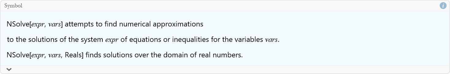
For higher orders, exact symbolic roots get messy. In WL we use NSolve[] to approximate the solution. Here we try another polynomial.

We can now compare this with NSolve. But how do we use NSolve?

Compare this with our symbolic solution.

We can see they are the same. Here is the plot of this curve.

So, we see five crossings—rare for a quintic, as complex roots often dominate. NSolve[] shines when Solve[]’s symbolic output is unwieldy.

Workflow for Higher Orders

Try Solve[] for symbolic roots; switch to NSolve[] for numbers.

Plot to visualize real roots—higher degrees mean more twists.

Terms and Definitions

Term/Definition 8.31 Higher-order equation: A polynomial equation of degree greater than 2 (e.g., quintic degree 5, sextic degree 6, etc.).

Term/Definition 8.32 Quintic equation: A polynomial equation of degree 5 in the general form .

Term/Definition 8.33 NSolve[] (Wolfram Language function): A command that finds numerical approximations to roots of equations (used when symbolic solutions are messy or complex).

Assumptions (the implicit beliefs the author relies on)

Assumption 8.23: Numerical approximation (NSolve[]) is acceptable when symbolic output is unwieldy.

Principles

Principle 8.18: Higher-order equations (degree > 4) have n roots — some real, many complex (Fundamental Theorem of Algebra).

Principle 8.19: No general algebraic formula exists for degree ≥ 5 (this is the Abel-Ruffini theorem) — rely on symbolic/numerical solving.

Exercise 8.17: Begin with Term/Definition 8.31 and copy it into your notebook. Reflect on its meaning for a few minutes. Note any thoughts that come to mind. How would you explain this to someone sitting in front of you. Write this down. Then do this for each term/definition, assumption, and principle.

Exercise 8.18
a) Find the roots of , then plot it.
b) Approximate the roots of , then plot it.
c) Calculate the discriminant of and find its roots.

Polynomial Manipulation

Polynomials are the workhorses of mathematics and physics. Manipulating polynomials lets you uncover their structure—roots, coefficients, or simplified forms. In Lesson 7, you learned to expand

(8.19)

to

(8.20)

and you learned to factor

(8.21)

into

(8.22)

Higher-degree polynomials just need more tools, and WL delivers.

Do you need a specific term’s coefficient? For the polynomial,

(8.23)

the coefficient for the third term (the term) is clearly -2. How do we get WL to do this?

We can use the Coefficient command.

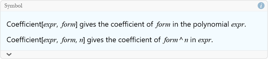
So, to find the coefficient would be given by the following command line.

We can also divide polynomials to simplify or find roots. Let’s say we want to divide

(8.24)

by

(8.25)

We use the command PolynomialQuotient.

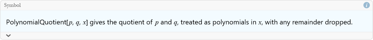
So the command line would be.

Is there a remainder? For this we use the command PolynomialRemainder.

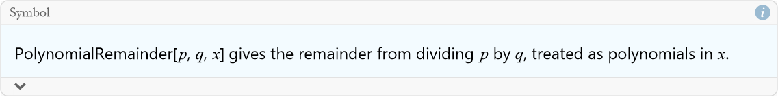
The command line would then be as follows:

Workflow for Polynomial Manipulation

Expand with Expand[] to see all terms.
Factor with Factor[] for roots or structure.
Simplify with Simplify[] to reduce.
Use Coefficient[] or PolynomialRemainder[] for specific insights.

Terms and Definitions

Term/Definition 8.34 Polynomial manipulation: The general process of transforming polynomials (expanding, factoring, simplifying, finding coefficients, dividing, etc.) to reveal structure, roots, or simplified forms.

Term/Definition 8.35 Coefficient[] (Wolfram Language function): Extracts the coefficient of a specific term (e.g., Coefficient[poly, x, 2] gives the coefficient).

Term/Definition 8.36 PolynomialQuotient[] (Wolfram Language function): Divides one polynomial by another and returns the quotient (remainder dropped).

Term/Definition 8.37 PolynomialRemainder[] (Wolfram Language function): Divides one polynomial by another and returns only the remainder.

Assumptions (the implicit beliefs the author relies on)

Assumption 8.24: Polynomial manipulation is essential for understanding structure, and finding roots.

Assumption 8.25: Polynomial division (Quotient and Remainder) works exactly like numerical long division.

Assumption 8.26: Remainder = 0 means exact division (divisor is a factor).

Principles

Principle 8.20: Polynomial division:  PolynomialQuotient[p, q, x] → quotient (remainder discarded).  

Principle 8.21: PolynomialRemainder[p, q, x] → remainder only.  

Principle 8.22: Quotient × divisor + remainder = original polynomial.

Exercise 8.19: Begin with Term/Definition 8.34 and copy it into your notebook. Reflect on its meaning for a few minutes. Note any thoughts that come to mind. How would you explain this to someone sitting in front of you. Write this down. Then do this for each term/definition, assumption, and principle.

Exercise 8.20
a) Find the coefficient for .
b) Divide by x-2 and find the remainder.
c) Factor and make a list of its coefficients.
d) Simplify , then plot the result.
e) Expand , then find its quotient when divided by x-1.

PolynomialReduce[]

Dividing polynomials might sound like a chore from algebra class, but the Wolfram Language (WL) makes it a breeze with PolynomialReduce[]. This function breaks a polynomial into a quotient and remainder when divided by another polynomial—think of it as long division. This command offers a systematic way to dissect polynomials of any degree, revealing their structure and roots.

Given a polynomial P(x) and a divisor D(x), PolynomialReduce[] is a go-to command.

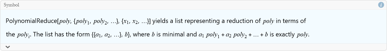
where we can think of this list of a terms as a polynomial, the quotient, and b is the remainder. This is more powerful than PolynomialQuotient[] and PolynomialRemainder[] alone—it gives both in one shot.

Say we want to use it to divide poly22 by poly23.

Let’s try one with a remainder.

Imagine a potential energy equation describing the displacement of a nonlinear system,

(8.26)

We want to see if x = 1 is a factor of (8.26).

We can clearly see that we have a remainder of -1, so x=1 is not a root of (8.26). We can solve this.

We can clearly see no roots at x=1. We can plot it to see the curve.

We see two crossings (equilibrium points) at x = -2.34 and 1.58. There are no roots at x=1.

Workflow with PolynomialReduce[]

Test divisors (e.g., x - a) to find factors/roots.
Check remainder: 0 means a root; nonzero adjusts the polynomial.
Factor quotients or solve remainders for all roots.
Plot to confirm visually.

Terms and Definitions

Term/Definition 8.38 PolynomialReduce[] (Wolfram Language function): A command that reduces a polynomial with respect to a list of divisor polynomials, returning a list of coefficients and a remainder (more powerful than PolynomialQuotient[] + PolynomialRemainder[] as it gives both in one step).

Assumptions (the implicit beliefs the author relies on)

Assumption 8.27: PolynomialReduce[] is a more comprehensive tool than separate use of PolynomialQuotient[] and PolynomialRemainder[].

Assumption 8.28: Remainder degree is always less than divisor degree(s) — standard polynomial division property.

Assumption 8.29: PolynomialReduce[] works for any degree and multiple divisors.

Principles

Principle 8.23: PolynomialReduce[poly, {div1, div2, ...}, x] reduces poly with respect to divisors, returning coefficients and remainder in one operation.

Principle 8.24: Output form: {{a1, a2, ...}, b} where poly = a1·div1 + a2·div2 + … + b (b = remainder).

Exercise 8.21: Begin with Term/Definition 8.38 and copy it into your notebook. Reflect on its meaning for a few minutes. Note any thoughts that come to mind. How would you explain this to someone sitting in front of you. Write this down. Then do this for each term/definition, assumption, and principle.

Exercise 8.22: Use PolynomialReduce[]:
a) Divide by t-1, and check the quotient and remainder.
b) Divide by x-2 and plot the original polynomial.
c) Reduce by v-1, then find its roots.
d) Divide by f-1 then plot the result.
e) Divide by x-1, then plot the result.

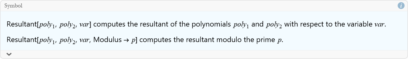
Resultant[]

When two polynomials intersect they might share roots, and the Wolfram Language (WL) gives us the Resultant[] command to find out without solving them fully. This command lets us see if two polynomials P(x) and Q(x) have common solutions—where P(x) = 0 and Q(x) = 0 at the same x. This isn’t just math trickery—it’s useful in physics, like checking when two system states align. Here, we’ll use Resultant[] to detect shared roots, tie it to polynomial manipulation, and see its practical side.

The resultant of two polynomials P(x) and Q(x) is a single number (or expression, if coefficients are symbolic) that’s zero if they have a common root. It’s especially handy when factoring or solving directly gets messy.

Let’s say we have this situation.

Why does this equal 0? If we solve this as a system of equations we can see the reason.

The two polynomials have a common root. We can plot this to make sure. We are going to use the PlotLegends command to specify which curve represents which solution.

What happens if the second polynomial is slightly different.

This tells us there are no common roots.

We can plot this.

We can see that the crossings don’t align with the horizontal axis—so we have two distinct roots.

Workflow for Resultant[]

Use Resultant[P, Q, x] to check for common roots.
If 0, solve both or factor to find shared ( x ).
If nonzero, roots differ—plot to visualize.
Pair with Solve[] or Factor[] for full insight.

Terms and Definitions

Term/Definition 8.39 Resultant[] (Wolfram Language function): A command that computes the resultant of two polynomials with respect to a variable; a single number (or expression) that is zero if and only if the polynomials share a common root.

Term/Definition 8.40 Resultant (mathematical concept): A value computed from two polynomials; zero when they have a common root (shared solution); non-zero otherwise.

Term/Definition 8.41 Common root: A value of x where both polynomials equal zero simultaneously (P(x) = 0 and Q(x) = 0).

Term/Definition 8.42 Common factor: A polynomial that divides both P(x) and Q(x); if they share a linear factor (x - c), then x = c is a common root.

Term/Definition 8.43 PlotLegends: An option in Plot[] to label multiple curves for clarity (e.g., PlotLegends → {poly1, poly2}).

Assumptions (the implicit beliefs the author relies on)

Assumption 8.30: Two polynomials share a common root if and only if their resultant is zero.

Assumption 8.31: The resultant is a complete algebraic test for common roots without needing to solve either polynomial fully.

Assumption 8.32: Plotting multiple polynomials together with legends shows visually whether they share roots (intersection points).

Principles

Principle 8.25: Use Resultant[poly1, poly2, x] to test for common roots: resultant = 0 means shared root(s); non-zero means no common roots.

Principle 8.26: Resultant is a single algebraic invariant — zero if and only if polynomials have a common factor/root.

Principle 8.27: Resultant is faster than full solving for detecting shared roots — especially useful for higher-degree polynomials.

Principle 8.28: Use Resultant[] as a diagnostic tool before full solving or factoring.

Principle 8.29: Plotting with legends clarifies which curve is which and highlights intersections.

Exercise 8.23: Begin with Term/Definition 8.39 and copy it into your notebook. Reflect on its meaning for a few minutes. Note any thoughts that come to mind. How would you explain this to someone sitting in front of you. Write this down. Then do this for each term/definition, assumption, and principle.

Exercise 8.24: Use Resultant[]:
a) Compute the resultant of and t-2, and plot the two polynomials.
b) Check for common roots between and x-1 and plot the polynomials.
c) Compute the resultant of by v-2, then visualize it.
d) Detect shared roots between and f-1 then plot the result.
e) Compute the resultant and x+1, then check the result.

Simplify with Assumptions

Simplifying expressions is a cornerstone of symbolic computation, and you’ve already seen the Wolfram Language (WL) function Simplify[] tame polynomials. But what if Simplify[] doesn’t know the full story—like whether a variable is positive or a parameter is real? That’s where the Assumptions option comes in, giving Simplify[] extra context to sharpen its results. This is like giving WL a hint to unlock simpler forms.

Simplify[] alone guesses what’s simplest based on general rules, but assumptions tell it specific conditions—like x > 0 or a is real—leading to more targeted outcomes. This is crucial in physics, where variables often have constraints (e.g., time is positive, mass is real), ensuring results match reality. We have already seen that the square root responds to assumptions.

Say that you have derived an expression the potential energy of a particle under a nonlinear force in terms of its displacement x and have this result,

(8.27)

You want to simplify this expression using Wolfram Language, assuming that x>1 (a physical constraint, you assume that the displacement is positive and beyond a certain point to avoid division by zero at x=1). You first define the potential,

You then try to simplify it with your assumptions.

We are left with the quadratic expression . We can plot this.

Terms and Definitions

Term/Definition 8.44 Assumptions (option in Simplify[]): A directive that provides additional context or constraints to guide simplification (e.g., x > 1, x ≠ 1, real parameters); can be a single condition or a list/logical combination.

Assumptions(the implicit beliefs the author relies on)

Assumption 8.33: Symbolic simplification (Simplify[]) can be made more accurate and physically meaningful by providing constraints via the Assumptions option.

Assumption 8.34: Physical constraints (e.g., displacement x > 1 to avoid division by zero at x = 1) are common in real-world problems and should guide computation.

Assumption 8.35: Wolfram Language respects logical combinations in Assumptions (e.g., x > 1 && x ≠ 1) to avoid invalid domains.

Principles

Principle 8.30: Assumptions can include inequalities (x > 1), exclusions (x ≠ 1), or logical combinations (&&, ||).

Principle 8.31: Provide assumptions to avoid singularities (e.g., denominators ≠ 0) and get simpler, relevant forms.

Principle 8.32: Simplify rational expressions under constraints: WL cancels common factors and respects domain limits.

Principle 8.33: Physical meaning guides assumptions: e.g., displacement x > 1 to stay away from x = 1 singularity.

Exercise 8.25: Begin with Term/Definition 8.44 and copy it into your notebook. Reflect on its meaning for a few minutes. Note any thoughts that come to mind. How would you explain this to someone sitting in front of you. Write this down. Then do this for each term/definition, assumption, and principle.

Exercise 8.26: Simplify
a) with the assumption t>0.:
b) with the assumption x>1 and plot the result.
c) assuming v>0, then visualize it.
d) assuming f>2 then plot the result.
e) assuming x>1, then plot the result.

Summary

Write a summary of this lesson as an exercise.

For Further Study

I. M. Gelfand, A. Shen, (1993), Algebra, Birkhauser. As stated in Lesson 4a, I can think of few that are better.

Navy Education and Training Professional Development and Technology Center, (1980) Mathematics, Basic Math and Algebra, NAVEDTRA 144139, Reprinted in 1985 (available for free at the Internet Archive https://archive.org/details/US_Navy_Training_Course_-_Mathematics_Basic_Math_and_Algebra). This is the first of a comprehensive set of manuals for training sailors in basic math.

Bruce F. Torrence, Eve A. Torrence, (2019), The Student’s Introduction to Mathematica and the Wolfram Language, Cambridge University Press, 3rd Edition