Lesson 7: Quadratic Equations
“Not a lot of people know this, but I’m very good at mathematics. When I was an angry teenager, I used to sit in my room and do quadratic equations to calm myself down.” – Samantha Bond
“It’s not for nothing that advanced mathematics tend to be invented in hot countries. It’s because of the morphic resonance of all the camels who have that disdainful expression and famous curled lip as a natural result of an ability to do quadratic equations.” – Terry Pratchett
Introduction
Unlike the linear equations of the previous chapter, which involved variables raised only to the first power (like x), the equations we study in this lesson involve variables raised to the second power (think ![]() ). We call these terms quadratic terms. Equations with such terms are called quadratic equations. They’re the next rung on our ladder toward understanding the mathematics that underpins theoretical physics.
). We call these terms quadratic terms. Equations with such terms are called quadratic equations. They’re the next rung on our ladder toward understanding the mathematics that underpins theoretical physics.
Quadratic Equations
Now that we’ve set the stage, let’s get to the heart of the matter. What, exactly, is a quadratic equation? At its core, a quadratic equation is a mathematical statement that involves a variable raised to the second power. While a linear equation like
![]()
(7.1)
describes a straight line, a quadratic equation opens the door to curves.
In its standard form a quadratic equation is written as
![]()
(7.2)
Here, x is the variable we’re solving for, and the coefficients a, b, and c are constants or parameters that define the equation’s behavior.
The term ![]() is the quadratic term, giving the equation its second-degree status. The b x term is the linear term, and c is the constant term. For example, in the equation
is the quadratic term, giving the equation its second-degree status. The b x term is the linear term, and c is the constant term. For example, in the equation
![]()
(7.3)
we have a = 3, b = -4, and c = 1. That little ![]() changes everything—it means we’re no longer dealing with a single, straight solution path but rather a pair of possibilities, as quadratics can have up to two solutions.
changes everything—it means we’re no longer dealing with a single, straight solution path but rather a pair of possibilities, as quadratics can have up to two solutions.
Why do quadratics matter in physics? Imagine a ball tossed into the air. Its height over time doesn’t follow a straight line—it rises, slows, and falls back down, tracing a parabolic arc. That motion is represented by a quadratic equation, where the height depends on time squared. Or consider a spring oscillating under a force that grows with distance squared—another quadratic relationship. These equations let us model systems with acceleration, curvature, and energy in ways linear equations simply can’t.
The solutions to a quadratic equation—called its roots—tell us where the parabola crosses the horizontal-axis (if it does at all). Sometimes there are two distinct roots, sometimes one (a perfect hit at the vertex), and sometimes none in the real number world (imagine a parabola that never dips below the axis). This variety makes quadratics both intriguing and powerful.
In the sections that follow, we’ll learn how to find these roots using techniques like factoring, completing the square, and the quadratic formula. But for now, let’s get comfortable with the idea that quadratic equations are our gateway to describing a universe that’s rarely flat or simple. They’re the mathematical language of arches, orbits, and motion—and they’re about to become your new best friend.
Terms and Definitions
Term/Definition 7.1 Quadratic equation: A mathematical equation where the highest power of the variable is 2; standard form ![]() .
.
Term/Definition 7.2 Quadratic term: The term with the variable raised to the second power (![]() ).
).
Term/Definition 7.3 Linear term: The term with the variable raised to the first power (b x).
Term/Definition 7.4 Constant term: The term with no variable (c).
Term/Definition 7.5 Roots (of a quadratic equation): The values of x that satisfy the equation; up to two real roots are possible.
Assumptions (the implicit beliefs the author relies on)
Assumption 7.1: The standard form ![]() fully captures the general quadratic equation.
fully captures the general quadratic equation.
Assumption 7.2: Quadratic equations can have zero, one, or two real roots.
Exercise 7.1: Begin with Term/Definition 7.1 and copy it into your notebook. Reflect on its meaning for a few minutes. Note any thoughts that come to mind. How would you explain this to someone sitting in front of you. Write this down. Then do this for each term/definition and assumption.
Seeing a Quadratic Equation
Before we dive into the nuts and bolts of solving quadratic equations, let’s take a step back and see what they look like. In mathematics, a quadratic equation is a particular arrangement of symbols, we can call it a mathematical structure. It needs to have no other meaning than the symbols. In a real-world application, a quadratic equation isn’t just a string of symbols—it’s a shape, a story, and a key to understanding. Picture a ball soaring through the air, its path traces a curve called a parabola, and that curve comes from a quadratic equation. Let’s explore this visual side to get a feel for what we’re working with.
It is not obvious, at first glance, that a quadratic equation, like ![]() , describes a parabola when you graph it. Here’s what that means. The coefficient a controls the direction and “steepness.” If a > 0, then the parabola opens upward (like a U); if a < 0, it opens downward (like an upside-down U). The coefficient b shifts the curve left or right and also can change its tilt. The factor c lifts or lowers the whole parabola—think of it as the starting height.
, describes a parabola when you graph it. Here’s what that means. The coefficient a controls the direction and “steepness.” If a > 0, then the parabola opens upward (like a U); if a < 0, it opens downward (like an upside-down U). The coefficient b shifts the curve left or right and also can change its tilt. The factor c lifts or lowers the whole parabola—think of it as the starting height.
The graph’s shape tells us a lot. First, it shows us where it crosses the horizontal-axis (the roots), its highest or lowest point (the vertex), and how it behaves.
Imagine the equation,
![]()
where (according to (7.2)) a = -1 (downward opening). b = 4, and c = 0.
If you plot this (or picture it), it starts at (0, 0), climbs to a peak, then drops back to zero. Where it hits y = 0 shows us the roots. Set
![]()
as we will see from methods below, this has roots at x = 0 and x = 4—the curve begins and ends there, with a peak in between.
With the Wolfram Language from earlier lessons, we can visualize this.
![]()
You’ll see a downward-opening parabola crossing the horizontal-axis at 0 and 4, peaking around x = 2. The vertex—the highest point—is key.
Seeing the parabola sets up everything. It allows us to find the roots, to see the vertex, and see the direction. That parabola isn’t just a graph—it’s a projectile’s arc.
Terms and Definitions
Term/Definition 7.6 Parabola: The graph of a quadratic equation; a U-shaped curve (opens up if a > 0, down if a < 0).
Term/Definition 7.7 Roots (of quadratic): The x-values where the equation equals zero (where parabola crosses x-axis); up to two real roots.
Term/Definition 7.8 Vertex: The highest or lowest point on the parabola (turning point); located at x = -b/(2a).
Term/Definition 7.9 Direction (of parabola): Opens upward (a > 0, minimum at vertex) or downward (a < 0, maximum at vertex).
Term/Definition 7.10 Plot (in WL): The command to graph a function or equation over a range (e.g., Plot[expression, {x, xmin, xmax}]).
Assumptions (the implicit beliefs the author relies on)
Assumption 7.3: Graphing quadratics reveals key features: roots (crossings), vertex (peak/trough), direction (up/down).
Assumption 7.4: The coefficient a determines direction and steepness; b shifts/tilts; c shifts vertically.
Assumption 7.5: Plotting a few points or using WL Plot reveals the full parabolic shape and behavior.
Principles
Principle 7.1: Quadratic equations produce parabolic graphs.
Principle 7.2: Standard form ![]() : The coefficient a controls direction (positive = up, negative = down) and steepness; b shifts left/right and tilts;
: The coefficient a controls direction (positive = up, negative = down) and steepness; b shifts left/right and tilts;
c shifts up/down (y-intercept).
Exercise 7.2: Begin with Term/Definition 7.6 and copy it into your notebook. Reflect on its meaning for a few minutes. Note any thoughts that come to mind. How would you explain this to someone sitting in front of you. Write this down. Then do this for each term/definition, assumption, and principle.
Exercise 7.3: Plot the following quadratic equations:
a) ![]() . Estimate the values of the roots and the vertex.
. Estimate the values of the roots and the vertex.
b) ![]() for x=-2 to x=2. Are there any real roots?
for x=-2 to x=2. Are there any real roots?
c) ![]() for x=-1 to x=5. Estimate the vertex.
for x=-1 to x=5. Estimate the vertex.
Exercise 7.4: Plot both ![]() and
and ![]() for x=-3 to x=3. How does it change due to the linear term (2x)?
for x=-3 to x=3. How does it change due to the linear term (2x)?
Exercise 7.5: Plot ![]() ,
,![]() , and
, and ![]() for x=-2 to x=2. How does changing the coefficient alter the shape and direction?
for x=-2 to x=2. How does changing the coefficient alter the shape and direction?
The Number of Roots, the Discriminant, and the Vertex
When we examine a quadratic equation, whose general form is ![]() we ask how many roots does a quadratic equation have? This is where things get interesting. Quadratic equations can have zero, one, or two real roots, depending on the relationship between a, b, and c. To see why, imagine the graph of a quadratic—a parabola that curves through space. The roots are the points where this parabola crosses the horizontal-axis. Let’s break it down into the possible cases:
we ask how many roots does a quadratic equation have? This is where things get interesting. Quadratic equations can have zero, one, or two real roots, depending on the relationship between a, b, and c. To see why, imagine the graph of a quadratic—a parabola that curves through space. The roots are the points where this parabola crosses the horizontal-axis. Let’s break it down into the possible cases:
Two Real Roots: If the parabola crosses the horizontal-axis at two distinct points, the equation has two solutions. Take ![]() . Its roots are (as using the methods described below) x = 1 and x = 2, reflecting a parabola that soars above the horizontal axis and descends back down.
. Its roots are (as using the methods described below) x = 1 and x = 2, reflecting a parabola that soars above the horizontal axis and descends back down.
One Real Root: If the parabola just grazes the horizontal-axis at a single point (its vertex), there’s only one root. For example, ![]() has a single root at x = 1, where the parabola kisses the axis before curving away.
has a single root at x = 1, where the parabola kisses the axis before curving away.
Zero Real Roots: If the parabola never touches the horizontal-axis—say, it opens upward and sits entirely above it—there are no real roots. Consider ![]() . Solving this gives only imaginary solutions (x = i or x = -i), but no real numbers work.
. Solving this gives only imaginary solutions (x = i or x = -i), but no real numbers work.
What decides this fate? The key lies in a quantity called the discriminant, defined as
![]()
(7.4)
The discriminant acts like a crystal ball for the number of roots. If D > 0, there are two distinct real roots. If D = 0, there’s exactly one real root. And, if D < 0, there are no real roots at all (though complex roots exist, which we’ll touch on later).
For instance, in
![]()
(7.5)
we calculate
![]()
(7.6)
Since D > 0, we expect two roots (and indeed, we find x = 1 and x = 3). Compare this to
![]()
(7.7)
where
![]()
(7.8)
signaling that there are no real roots.
You can also calculate the vertex of (7.5),
![]()
(7.9)
What does this tell us? We know that we have a parabola that opens downward (b=-4), has a maximum value of 2, and intersects the horizontal axis twice.
Terms and Definitions
Term/Definition 7.11 Two real roots: The case where the parabola crosses the horizontal axis at two distinct points.
Term/Definition 7.12 One real root: The case where the parabola touches the horizontal axis at exactly one point (the vertex).
Term/Definition 7.13 Zero real roots: The case where the parabola never crosses the horizontal axis (no real solutions; complex roots exist).
Term/Definition 7.14 Discriminant (symbol D): The quantity ![]() that determines the nature and number of real roots of a quadratic equation.
that determines the nature and number of real roots of a quadratic equation.
Assumptions (the implicit beliefs the author relies on)
Assumption 7.6: The number and nature of real roots are completely determined by the discriminant ![]() .
.
Assumption 7.7: The sign of a determines the parabola’s direction (upward for a > 0, downward for a < 0).
Assumption 7.8: The vertex formula x = -b / (2a) always locates the turning point correctly.
Assumption 7.9: Complex roots exist when D < 0 but are not considered “real” solutions in this context.
Principles
Principle 7.3: The discriminant ![]() determines the number of real roots: D > 0 → two distinct real roots, D = 0 → exactly one real root (repeated root at vertex), and D < 0 → no real roots (two complex roots).
determines the number of real roots: D > 0 → two distinct real roots, D = 0 → exactly one real root (repeated root at vertex), and D < 0 → no real roots (two complex roots).
Principle 7.4: The parabola’s graph visually shows roots (crossings of x-axis) and vertex (peak or trough).
Principle 7.5: The vertex x-coordinate formula: ![]() ; locates the axis of symmetry (the midpoint of the parabola).
; locates the axis of symmetry (the midpoint of the parabola).
Principle 7.6: Use discriminant to quickly predict root behavior before solving fully.
Principle 7.7: Graphing (or visualizing) quadratics reveals behavior that algebra alone may not show immediately.
Principle 7.8: Real roots exist when D ≥ 0; zero real roots mean the parabola never crosses the axis (no real solutions).
Exercise 7.6: Begin with Term/Definition 7.11 and copy it into your notebook. Reflect on its meaning for a few minutes. Note any thoughts that come to mind. How would you explain this to someone sitting in front of you. Write this down. Then do this for each term/definition, assumption, and principle.
Solution by Factoring
Now that we’ve explored the structure of quadratic equations and their roots, it’s time to roll up our sleeves and learn how to solve them. One of the most intuitive methods is factoring—breaking the equation into simpler pieces that reveal its solutions directly. This approach works best when the quadratic can be neatly split into factors, and it’s a great starting point before we tackle more complicated tools like the quadratic formula. Let’s dive in and see how it works.
A quadratic equation in standard form is
![]()
(7.10)
The goal of factoring is to rewrite the left side as a product of two binomials—that, when multiplied, give us the original equation. If we can write it as
![]()
(7.11)
then the solutions (or roots) come from setting each factor to zero
![]()
(7.12)
or
![]()
(7.13)
This relies on a key property, if the product of two numbers is zero, at least one of them must be zero.
Consider the equation
![]()
(7.14)
Here, a = 1, b = -5, and c = 6. We need two numbers that multiply to 6 (the constant term, c) and add to -5 (the coefficient of x, b). Let’s test some pairs, 1·6 = 6, but 1 + 6 = 7 (too big). Try 2 · 3 = 6, and 2 + 3 = 5 (close, but we need -5). Try -2 · -3 = 6, and -2 + -3 = -5 (perfect!). So, we factor the equation as,
![]()
(7.15)
We now check it by expanding
![]()
(7.16)
this matches our original. Now, set each factor to zero,
![]()
(7.17)
and,
![]()
(7.18)
So, the roots are x = 2 and x = 3. To verify, plug them back in to (7.15). For x = 2,
![]()
(7.19)
For x = 3,
![]()
(7.20)
Both check out!
Let’s try another,
![]()
(7.21)
Here, a = 2, b = 7, and c = -4. Since a≠1, it’s trickier—we need numbers that multiply to
![]()
(7.22)
and add to b = 7. Let’s test some pairs,
![]()
(7.23)
and 8 + (-1) = 7, so this works!
We rewrite the middle term using these numbers
![]()
(7.24)
Now we group and factor this,
![]()
(7.25)
We can then check this,
![]()
(7.26)
Good! Now we solve for the identified binomial factors,
![]()
(7.27)
and
![]()
(7.28)
We then verify these results. For ![]() ,
,
![]()
(7.29)
For x = -4,
![]()
(7.30)
So, both roots hold.
Factoring works beautifully when the numbers align, often signaled by a positive discriminant (![]() ) and integer-friendly coefficients. Not every quadratic factors easily, though. For now, factoring is your first step to cracking the quadratic code—simple, elegant, and deeply satisfying.
) and integer-friendly coefficients. Not every quadratic factors easily, though. For now, factoring is your first step to cracking the quadratic code—simple, elegant, and deeply satisfying.
Terms and Definitions
Term/Definition 7.15 Splitting the middle term: A technique for factoring quadratics ![]() by decomposing bx into two terms whose coefficients multiply to a·c and add to b.
by decomposing bx into two terms whose coefficients multiply to a·c and add to b.
Term/Definition 7.16 Grouping: A factoring method for polynomials with four or more terms; group in pairs, factor GCF from each pair, then factor common binomial.
Term/Definition 7.17 Trial and error: Trying different possible factor pairs to match the original polynomial.
Term/Definition 7.18 Conjugate product: The product of a complex number and its conjugate (e.g., ![]() ).
).
Assumptions (the implicit beliefs the author relies on)
Assumption 7.10: Factoring is a primary, intuitive method for solving quadratics when it works.
Assumption 7.11: Many quadratics factor nicely over integers or rationals (especially with integer coefficients).
Assumption 7.12: If a quadratic factors into binomials, roots come directly from setting each factor to zero.
Assumption 7.13: The zero-product property holds: if (p x + q)(r x + s) = 0, then p x + q = 0 or r x + s = 0.
Assumption 7.14: Sum of squares is irreducible over reals but factors over complexes using conjugates.
Assumption 7.15: Difference of squares, sum/difference of cubes, and perfect square trinomials are reliable patterns.
Assumption 7.16: Splitting middle term and grouping cover most integer-coefficient quadratics.
Assumption 7.17: Trial and error is viable when coefficients are small and factors are integers.
Assumption 7.18: Some quadratics are irreducible over reals; complex roots may be needed.
Assumption 7.19: Verification (plugging roots back in to the original equation) confirms correct factoring and solutions.
Principles
Principle 7.9: Factoring rewrites quadratics as products → roots from setting factors = 0.
Principle 7.10: Start with GCF: factor out common factor from all terms.
Principle 7.11: Use zero-product property: product = 0 implies at least one factor = 0.
Exercise 7.7: Begin with Term/Definition 7.15 and copy it into your notebook. Reflect on its meaning for a few minutes. Note any thoughts that come to mind. How would you explain this to someone sitting in front of you. Write this down. Then do this for each term/definition, assumption, and principle.
Exercise 7.8: Solve each equation by factoring and then plot the equations to verify your answers.
a) ![]() .
.
b) ![]() .
.
c) ![]() .
.
d) ![]() .
.
e) ![]() .
.
f) ![]() .
.
Solution by Completing the Square
Sometimes an attempt to factor a quadratic becomes very difficult. In such cases we can use a second technique. This technique not only helps us solve equations but also lays the groundwork for understanding concepts like parabolas and even trajectories in physics—think of a ball’s arc through the air! It’s a bit like sculpting: we reshape the equation into a form that reveals its solutions naturally.
Completing the square transforms a quadratic equation from its standard form,
![]()
(7.31)
into a perfect square trinomial plus a constant. Why? Because a perfect square, like ![]() , is easy to solve. This method works for any quadratic equation, even when factoring isn’t obvious, making it a versatile tool in your mathematical toolkit.
, is easy to solve. This method works for any quadratic equation, even when factoring isn’t obvious, making it a versatile tool in your mathematical toolkit.
Let’s solve a general quadratic equation, ![]() , by completing the square. Don’t worry—we’ll follow with a concrete example to make it crystal clear. We begin by moving the constant term. This allows us to start to isolate x. We accomplish this by subtracting c from both sides,
, by completing the square. Don’t worry—we’ll follow with a concrete example to make it crystal clear. We begin by moving the constant term. This allows us to start to isolate x. We accomplish this by subtracting c from both sides,
![]()
(7.32)
Divide by the leading coefficient. This always transforms the leading coefficient to 1,
![]()
(7.33)
To form a perfect square we need to find the magic number, take the coefficient of x (this is now ![]() ), halve it, and square it,
), halve it, and square it,
![]()
(7.34)
This is the number we’ll add to both sides to “complete” the square.
![]()
(7.35)
Rewrite the left as a square since the left side is now a perfect square trinomial and we can factor it,
![]()
(7.36)
We now simplify the right-hand side. We combine the terms on the right over a common denominator (![]() ),
),
![]()
(7.37)
So the equation becomes,
![]()
(7.38)
We then solve for x and we take the square root of both sides,
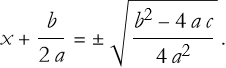
(7.39)
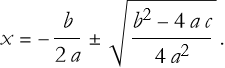
We must then isolate (x),

(7.40)
As it happens, this is the quadratic formula, and we will see more about this in the next section! Completing the square is actually how that famous formula is derived—pretty neat, right?
For example, solving
![]()
(7.41)
First, we move the constant,
![]()
(7.42)
Then we divide by 2,
![]()
(7.43)
Find the magic number. The coefficient of x is 4. Half of 4 is 2, and ![]() = 4. We add this to both sides,
= 4. We add this to both sides,
![]()
(7.44)
Rewrite this as a square,
![]()
(7.45)
Take the square root,
![]()
(7.46)
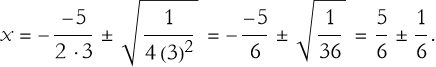
Solve for x,
![]()
(7.47)
So x=1 or x=-5. We can check this. For x = 1,
![]()
(7.48)
For x = -5,
![]()
(7.49)
Both work!
Completing the square isn’t just a trick—it’s a window into the geometry of quadratics. That ![]() form shows the vertex of a parabola, which could represent the peak height of a projectile in physics. Plus, it’s a stepping stone to the quadratic formula, which we’ll explore next. Practice this method, and you’ll see patterns emerge that connect algebra to the real world.
form shows the vertex of a parabola, which could represent the peak height of a projectile in physics. Plus, it’s a stepping stone to the quadratic formula, which we’ll explore next. Practice this method, and you’ll see patterns emerge that connect algebra to the real world.
Terms and Definitions
Term/Definition 7.19 Completing the square: A method to rewrite a quadratic equation as a perfect square trinomial plus a constant, revealing roots and vertex.
Term/Definition 7.20 Magic number (or completion term): The value added to both sides to form a perfect square; found by halving the linear coefficient and squaring it (![]() ).
).
Assumptions (the implicit beliefs the author relies on)
Assumption 7.20: Completing the square works for any quadratic equation (even when factoring is difficult or impossible over integers).
Assumption 7.21: The method reveals both algebraic solutions (roots) and geometric insight (vertex form).
Assumption 7.22: The “magic number” (![]() ) always completes the square when the leading coefficient is 1 (or after dividing by a).
) always completes the square when the leading coefficient is 1 (or after dividing by a).
Assumption 7.23: Verification by substitution is necessary to confirm solutions.
Principles
Principle 7.12: Completing the square transforms ![]() into vertex form:
into vertex form: ![]() .
.
Principle 7.13: Steps for completing the square:
Move constant term to right.
Divide by leading coefficient a to make leading term ![]() .
.
Add magic number ![]() to both sides.
to both sides.
Rewrite left as perfect square.
Simplify right side.
Take square root of both sides (include ±).
Solve for x.
Exercise 7.9: Begin with Term/Definition 7.19 and copy it into your notebook. Reflect on its meaning for a few minutes. Note any thoughts that come to mind. How would you explain this to someone sitting in front of you. Write this down. Then do this for each term/definition, assumption, and principle.
Exercise 7.10: Solve each equation by completing the square and then plot the equations to verify your answers.
a) ![]() .
.
b) ![]() .
.
c) ![]() .
.
d) ![]() .
.
e) ![]() .
.
Solution by the Quadratic Formula
After factoring and completing the square, we arrive at the superstar of quadratic-solving methods: the quadratic formula. This is the go-to tool when factoring feels like hunting for a needle in a haystack, or when completing the square gets tedious. It’s a universal key that unlocks the solutions to any quadratic equation. Let’s see how it works.
For a quadratic equation in standard form,
![]()
(7.50)
the solutions (or roots) are given by the formula,
(7.51)
This formula might look intimidating, but it’s just the result of completing the square on the general form—we did the heavy lifting in the last section! Now, it’s a plug-and-play solution.
Here is how it works. You begin by identifying a, b, and c by matching your equation to (7.51). Then we must compute the discriminant ![]() . Then you plug these values into the formula (7.51). Then you solve for the two values of x.
. Then you plug these values into the formula (7.51). Then you solve for the two values of x.
For example, solving
![]()
(7.52)
We begin by identifying the coefficients; a = 3, b = -5, and c = 2. Then we compute the discriminant,
![]()
(7.53)
Plug into the formula (7.52),
(7.54)
So, the solutions are x = 1 and ![]() . We can check this,
. We can check this,
![]()
(7.55)
and
![]()
(7.56)
Both hold!
The quadratic formula is like a Swiss Army knife—it works every time, no matter the equation. Memorize it, practice it, and you’ll see it pop up everywhere in physics.
Terms and Definitions
Term/Definition 7.21 Quadratic formula: The general solution for any quadratic equation ![]() ; given by
; given by![]() . Here the ± indicates two possible solutions: one with addition, one with subtraction of the square root term.
. Here the ± indicates two possible solutions: one with addition, one with subtraction of the square root term.
Assumptions (the implicit beliefs the author relies on)
Assumption 7.24: Every quadratic equation (![]() ) can be solved using the quadratic formula.
) can be solved using the quadratic formula.
Assumption 7.25: The quadratic formula is derived from completing the square on the general form.
Assumption 7.26: Roots can be real or complex; the formula works in all cases.
Assumption 7.27: Verification by substitution is necessary to confirm solutions.
Principles
Principle 7.14: Compute discriminant ![]() first: D > 0 → two distinct real roots, D = 0 → one real root (repeated), D < 0 → no real roots (complex conjugate pair).
first: D > 0 → two distinct real roots, D = 0 → one real root (repeated), D < 0 → no real roots (complex conjugate pair).
Principle 7.15: Plug a, b, c into formula; handle ± for both solutions.
Principle 7.16: Simplify square root and fraction step-by-step.
Exercise 7.11: Begin with Term/Definition 7.21 and copy it into your notebook. Reflect on its meaning for a few minutes. Note any thoughts that come to mind. How would you explain this to someone sitting in front of you. Write this down. Then do this for each term/definition, assumption, and principle.
Exercise 7.12: Solve each equation using the quadratic formula, find the discriminant, and then plot the equations to verify your answers.
a) ![]() .
.
b) ![]() .
.
c) ![]() .
.
d) ![]() .
.
e) ![]() .
.
Ballistic Trajectories
Quadratic equations aren’t just abstract puzzles—they can be used to describe the world around us, especially in physics. One powerful example is a ballistic trajectory: the curved path of an object—like a thrown ball, a kicked soccer ball, or even a cannonball—moving under gravity alone. What arc do you see? It’s a parabola, and its equation is quadratic. Let’s explore how the tools we’ve learned help us predict where and when that object lands.
Imagine you toss a ball straight up or at an angle. Once it leaves your hand, gravity pulls it back down, and its height over time follows a quadratic equation. For simplicity, let’s focus on vertical motion first (no horizontal wind or spin—just up and down). The height h(t) of the ball at time t is given by
![]()
(7.57)
where g is the acceleration due to gravity near the surface of the Earth (about 9.8 m ![]() ),
), ![]() is the initial speed (this is 0 if we simply drop something),
is the initial speed (this is 0 if we simply drop something), ![]() is the initial height, and t is the time. This is a quadratic equation in t, with coefficients
is the initial height, and t is the time. This is a quadratic equation in t, with coefficients ![]() ,
, ![]() , and
, and ![]() . The negative a means the parabola opens downward—makes sense, since gravity pulls the ball back to Earth.
. The negative a means the parabola opens downward—makes sense, since gravity pulls the ball back to Earth.
When does the ball hit the ground? That’s when h(t) = 0. So, we set the equation to zero and solve,
![]()
(7.58)
Let’s use the quadratic formula,
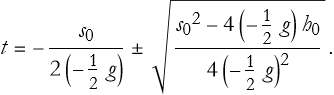
(7.59)
Suppose you throw a ball upward from a height of 2 m ![]()
![]() with an initial speed
with an initial speed ![]() m
m ![]() ), and the acceleration due to gravity is g=9.8 m
), and the acceleration due to gravity is g=9.8 m ![]() . When does it hit the ground?
. When does it hit the ground?
We write the equation,
![]()
(7.60)
Then we set h(t)=0, and simplify,
![]()
(7.61)
We then identify the coefficients, a = -4.9, b = 10, and c = 2.
Then compute the discriminant,
![]()
(7.62)
Then apply the quadratic formula,

(7.63)
So we have two approximate values of t, 2.2432 and -0.1835. Since negative time doesn’t really mean anything (since we can’t really consider a time before we begin measuring it), the answer is t≈2.2432 seconds.
Terms and Definitions
Term/Definition 7.22 Ballistic trajectory: The curved path of an object (e.g., thrown ball, cannonball) moving under gravity alone (no air resistance or other forces).
Term/Definition 7.23 Parabola: The shape of a ballistic trajectory when graphed (height vs. time); a quadratic curve.
Term/Definition 7.24 Height (symbol h(t)): The vertical position of the object at time t.
Term/Definition 7.25 Initial height (symbol ![]() ): The starting height of the object above a reference level (e.g., ground).
): The starting height of the object above a reference level (e.g., ground).
Term/Definition 7.26 Initial speed (symbol ![]() ): The starting vertical speed of the object (positive upward, zero if dropped).
): The starting vertical speed of the object (positive upward, zero if dropped).
Term/Definition 7.27 Acceleration due to gravity (symbol g): The constant downward acceleration near Earth’s surface (~9.8 m/s²).
Term/Definition 7.28 Time (symbol t): The elapsed time since release or launch.
Term/Definition 7.29 Height equation: The equation describing height over time in vertical motion under gravity: ![]() .
.
Assumptions (the implicit beliefs the author relies on)
Assumption 7.28: Objects in free fall (or projectile motion) experience constant downward acceleration g ≈ 9.8 ![]() .
.
Assumption 7.29: Motion is vertical only (straight up/down) or vertical component is isolated.
Assumption 7.30: Downward direction is negative (negative sign on g term in h(t)).
Assumption 7.31: Time t starts at 0 when object is released/launched.
Assumption 7.32: Negative time solutions are physically meaningless (discard them).
Principles
Principle 7.17: Ballistic trajectories are parabolic — height h(t) is a quadratic function of time: ![]() .
.
Principle 7.18: Negative leading coefficient (-(1/2) g) means parabola opens downward (object rises then falls).
Principle 7.19: Set h(t) = 0 to find time to hit ground (solve quadratic equation for t).
Principle 7.20: Height equation has two roots: one positive (physical landing time), one negative (discard — before t = 0).
Principle 7.21: Verify solution: substitute t back into h(t) to confirm ≈ 0 (accounting for rounding).
Principle 7.22: Gravity dominates vertical motion — produces characteristic parabolic arc.
Exercise 7.13: Begin with Term/Definition 7.22 and copy it into your notebook. Reflect on its meaning for a few minutes. Note any thoughts that come to mind. How would you explain this to someone sitting in front of you. Write this down. Then do this for each term/definition, assumption, and principle.
Using Solve[]
So far, we’ve tackled quadratic equations with factoring, completing the square, and the quadratic formula—great for understanding the math by hand. But what if you want a quick, reliable solution without the pencil-and-paper grind? Enter the Wolfram Language, which we introduced earlier, and its powerful function Solve[]. If you’ve used it for linear equations in Lesson 6, you’re ready to see how it handles quadratics—perfect for physics problems like our ballistic trajectories.
Recall that when we use solve, we write Solve[equation, variable to solve for]
Let’s see it in action.
We can first write the standard form.
![]()
This is equivalent to the quadratic formula (7.51).
Example 1: A Simple Quadratic
Take,
![]()
We could factor this to get (x-2)(x-3)=0.
![]()
![]()
This means that x = 2 and x = 3—exact roots, no fuss. Compare that to factoring by hand: same result, but Solve[] did it instantly.
Let’s revisit our ballistic example:
![]()
Of course, this matches our quadratic formula result from earlier. The negative root is before the throw, and the positive one (about 2.22 seconds) is when the ball lands.
Terms and Definitions
Term/Definition 7.30 Quadratic equation (in context): Equations of form a ![]() + b x + c == 0; solved symbolically by Solve[].
+ b x + c == 0; solved symbolically by Solve[].
Assumptions (the implicit beliefs the author relies on)
Assumption 7.33: WL handles quadratics exactly (no numerical approximation needed for these examples).
Principles
Principle 7.23: Use Solve[equation, variable] to solve any quadratic symbolically in WL.
Principle 7.24: Combine Solve[] with plotting (from prior sections) to visualize and verify solutions.
Exercise 7.14: Begin with Term/Definition 7.30 and copy it into your notebook. Reflect on its meaning for a few minutes. Note any thoughts that come to mind. How would you explain this to someone sitting in front of you. Write this down. Then do this for each term/definition, assumption, and principle.
Exercise 7.15: Solve each equation using Solve[] and then plot the equations to verify your answers.
a) ![]() .
.
b) ![]() .
.
c) ![]() .
.
d) ![]() .
.
e) ![]() .
.
Using Complex Numbers
Back in Lesson 3, we met complex numbers—those handy tools like 3 + 4i, where ![]() , that let us handle square roots of negatives. Now, in our quadratic journey, they’re about to shine. When a quadratic’s discriminant
, that let us handle square roots of negatives. Now, in our quadratic journey, they’re about to shine. When a quadratic’s discriminant ![]() dips below zero, real roots vanish, and complex roots take over. With our solving methods and Wolfram Language skills, we’ll see how these “imaginary” solutions come about.
dips below zero, real roots vanish, and complex roots take over. With our solving methods and Wolfram Language skills, we’ll see how these “imaginary” solutions come about.
For the general form of a quadratic ![]() , the quadratic formula gives,
, the quadratic formula gives,
![]()
(7.64)
If the discriminant is less than 0, ![]() , the square root becomes imaginary. This always yields two roots, often as conjugates (e.g., a + b i and a - b i). Let’s see it in action.
, the square root becomes imaginary. This always yields two roots, often as conjugates (e.g., a + b i and a - b i). Let’s see it in action.
Take the equation,
![]()
(7.65)
Comparing this to the standard form, we have a = 1, b = 4, and c = 5. The discriminant is then,
![]()
(7.66)
We apply this to the quadratic formula,
![]()
(7.67)
This gives us the roots, t = -2 + i and t = -2 - i. The parabola doesn’t hit the t-axis—complex roots tell us there’s no real solution here.
In Wolfram Language we write this:

![]()
Let’s tweak our ballistic equation. Suppose
![]()
there is no real landing time—physically, this might mean the conditions (speed, height) don’t allow a real trajectory under gravity alone. Complex roots wave a red flag that something’s off.
Terms and Definitions
Term/Definition 7.31 Complex roots: The solutions to a quadratic equation when the discriminant is negative; always come in conjugate pairs (e.g., -2 + i and -2 - i).
Assumptions (the implicit beliefs the author relies on)
Assumption 7.34: Quadratic equations always have two roots (counting multiplicity), either real or complex.
Principles
Principle 7.24: Quadratic formula always gives solutions: real when D ≥ 0, complex when D < 0.
Principle 7.25: Complex roots come in conjugate pairs (a + b i and a - b i) for real-coefficient quadratics.
Exercise 7.16: Begin with Term/Definition 7.31 and copy it into your notebook. Reflect on its meaning for a few minutes. Note any thoughts that come to mind. How would you explain this to someone sitting in front of you. Write this down. Then do this for each term/definition, assumption, and principle.
Exercise 7.17: Solve each equation using Solve[] and then plot the equations to verify your answers.
a) ![]() .
.
b) ![]() .
.
c) ![]() .
.
d) ![]() .
.
e) ![]() , where c=0, c=3, and c=-3.
, where c=0, c=3, and c=-3.
Summary
Write a summary of this lesson as an exercise.
For Further Study
I. M. Gelfand, A. Shen, (1993), Algebra, Birkhauser. As stated in Lesson 4a, I can think of few that are better.
Navy Education and Training Professional Development and Technology Center, (1980) Mathematics, Basic Math and Algebra, NAVEDTRA 144139, Reprinted in 1985 (available for free at the Internet Archive https://archive.org/details/US_Navy_Training_Course_-_Mathematics_Basic_Math_and_Algebra). This is the first of a comprehensive set of manuals for training sailors in basic math.