Lesson 6 Web

Lesson 6: Linear Equations

“It is impossible to be a mathematician without being a poet in soul.” Sofia Kovalevskaya

“Truth is ever to be found in simplicity, and not in the multiplicity and confusion of things.” Isaac Newton

Introduction

Linear equations are your gateway to mastering theoretical physics, letting you predict motion and balance forces with ease. In this lesson, you’ll explore what equations are, solve single-variable equations, revisit Ohm’s Law, balance forces, tackle systems of equations with substitution and elimination, and even plot graphs by hand and with Wolfram Language tools.

What is an Equation?

Forge connections between quantities with a mathematical statement that declares two expressions equal, linked by the equals sign =. This kind of expression, called an equation, captures relationships between numbers, variables, or both. Picture 2 + 3 = 5—a truth that stands firm. Now try x + 4 = 7. This challenges you to find the value of x that makes it true. Subtract 4 from both sides, and you reveal x = 3, solving the puzzle. In physics, such statements, like d = s t, tie distance, speed, and time, letting you pinpoint one when you know the others.

These relationships come in forms. Those with variables raised only to the power of 1, called linear equations, keep things direct and are our focus here. Others, like , add twists we’ll explore later. For now, solving these statements means making the expression on the left side equals match that on the right side.

In physics, these tools voice the universe’s rules. Newton’s second law, F = m a, binds force, mass, and acceleration. Rearrange it to a = F/m, and you can see that the action of a force on a mass is an acceleration of that mass. This ability to model reality fuels discovery.

These statements gain strength by restricting solutions to specific values, a concept we call constraints. For example, 5x = 10 yields one solution, x = 2, while x + y = 5 allows many pairs, like (1, 4) or (2, 3). By defining the values that satisfy the statement, constraints guide you to accurate answers. Embrace these boundaries to master linear equations and unlock physics problems.

What is an Equation?

Terms and Definitions

Term/Definition 6.1 Equation: A mathematical statement declaring two expressions equal, connected by the equals sign = (e.g., 2 + 3 = 5 or x + 4 = 7).

Term/Definition 6.2 Linear equation: An equation where variables are raised only to the power of 1 (no higher powers, squares, etc.); direct and solvable with basic operations.

Term/Definition 6.3 Solving an equation: The process of finding the value(s) of the variable(s) that make the equation true (e.g., subtracting 4 from both sides of x + 4 = 7 to get x = 3).

Term/Definition 6.4 Constraints: Restrictions or conditions that limit the possible solutions to an equation (e.g., 5x = 10 has one solution x = 2, while x + y = 5 allows infinitely many pairs).

Assumptions (the implicit beliefs the author relies on)

Assumption 6.1: Equality (two sides of = must be identical) is the core property of equations.

Assumption 6.2: Solving equations involves reversible operations (e.g., adding/subtracting the same value from both sides) that preserve equality.

Assumption 6.3: Physical laws (e.g., F = m a) are expressed as equations that can be rearranged to solve for any variable.

Assumption 6.4: Constraints are inherent in most physical problems (finite solutions, specific contexts).

Principles

Principle 6.1: Equations link quantities mathematically: left side equals right side (e.g., 2 + 3 = 5 is always true; x + 4 = 7 is true only for x = 3).

Principle 6.2: Use equations to solve for unknowns: perform identical operations on both sides to isolate the variable.

Principle 6.3: Rearrange equations to express relationships in different forms (e.g., d = s t → s = d / t → t = d / s).

Principle 6.4: Constraints define valid solutions: single solution for determined systems, multiple/infinite for underdetermined ones.

Principle 6.5: Embrace constraints as guides — they focus solutions and ensure physical relevance.

Exercise 6.1: Begin with Term/Definition 6.1 and copy it into your notebook. Reflect on its meaning for a few minutes. Note any thoughts that come to mind. How would you explain this to someone sitting in front of you. Write this down. Then do this for each term/definition, assumption, and principle.

Balancing Equations

When we ensure that both sides of an equation are actually equal, we say that we have balanced the equation. It’s about maintaining the equation’s truth by applying the same operation to each side simultaneously, a principle rooted in equality. For linear equations, this process is straightforward and essential for physics, where equations often describe measurable relationships.

Start with a basic example,

(6.1)

To isolate x, subtract 5 from both sides,

(6.2)

This simplifies to x = 7. The equation stays balanced because the same action—subtracting 5—applies everywhere. The key is to undo operations step-by-step: addition is reversed by subtraction, multiplication by division.

Consider the equation,

(6.3)

First, add 8 to both sides,

(6.4)

so,

(6.5)

Then, divide both sides by 3,

(6.6)

or,

(6.7)

Each move preserves balance, like adjusting a scale. For equations with variables on both sides,

(6.8)

Subtract 2x from both sides,

(6.9)

since 4 x - 2 x is just 2 x, we have

(6.10)

Now subtract both sides by 3.

(6.11)

(6.12)

Now we divide both sides by 2,

(6.13)

or,

(6.14)

The rule is simple, what you do to one side, do to the other.

Terms and Definitions

Term/Definition 6.5 Balancing an equation: The process of ensuring both sides of an equation remain equal by applying the same mathematical operation to each side simultaneously.

Term/Definition 6.6 Isolate the variable: The goal of solving an equation by performing operations to get the variable alone on one side (e.g., x = value).

Assumptions(the implicit beliefs the author relies on)

Assumption 6.5: An equation is a statement of equality that remains true only when both sides are equal.

Assumption 6.6: Equality is preserved when identical operations are applied to both sides of an equation.

Assumption 6.7: Linear equations (variables to power 1 only) can be solved by step-by-step reversal of operations. Addition is reversed by subtraction; multiplication is reversed by division (and vice versa).

Assumption 6.8: Operations can be performed on either side without changing the equation's validity, as long as they are identical.

Assumption 6.9: Solving involves undoing operations step-by-step until the variable is isolated.

Principles

Principle 6.6: Perform operations systematically: First handle addition/subtraction terms (add/subtract constants). Then handle multiplication/division (divide/multiply by coefficients).

Principle 6.7: Always verify solutions by substituting back into the original equation (implicit in balancing examples).

Exercise 6.2: Begin with Term/Definition 6.5 and copy it into your notebook. Reflect on its meaning for a few minutes. Note any thoughts that come to mind. How would you explain this to someone sitting in front of you. Write this down. Then do this for each term/definition, assumption, and principle.

Solving Single Variable Equations

In physics, we often encounter situations where we need to find an unknown variable that satisfies a given relationship. These relationships are expressed as equations, and solving them is a fundamental skill. In this section, we’ll focus on linear equations that involve just one unknown; what we call single-variable linear equations.

A single-variable linear equation is an equation that can be written in the general form,

(6.15)

Here, x is the variable we want to solve for, while a, b, and c are treated constants. A note must be added here. in some cases the are true constants while in others they are constant only for the problem at hand, we call such symbols parameters. For example:

(6.16)

Our goal in solving the equation is to find the value of x that makes this statement true.

The art of solving an equation is like the balancing we did in the previous section. Whatever you do to one side, you must do to the other to keep the equation true. In effect what are are trying to do here is to isolate the variable we want to find on one side of the equation (traditionally this is the left-hand side). In linear equations in general we’ll use two main operations to isolate our variable: Addition or subtraction to move terms, and multiplication or division to simplify coefficients.

Let’s break it down step by step.

Identify the goal: Get the variable by itself on one side of the equation.

Eliminate constants: Add or subtract terms to move everything except variable-related terms to the other side.

Isolate the variable: Divide or multiply to remove any coefficient attached to the variable.

Check your work: Plug the solution back into the original equation to verify that it holds.

For example, consider equation (6.16),

(6.17)

Step 1: Our goal is to solve for x.

Step 2: Subtract 3 from both sides to remove the constant on the left, here we introduce the symbol ⇒ for the phrase, “This leads to the conclusion...”.

(6.18)

Step 3: Divide both sides by 2 to isolate x,

(6.19)

Step 4: Verify,

(6.20)

The equation holds true, so x = 2 is the correct solution.

Here is another example,

(6.21)

Step 1: We want to isolate x.

Step 2: Subtract 5 from both sides:

(6.22)

Step 3: Divide both sides by -3 (note that dividing by a negative keeps the balance),

(6.23)

Step 4: Verify,

(6.24)

So we have solved this one, too.

Equations like these pop up in physics all the time. Suppose you’re calculating the speed of an object under constant acceleration. The equation might look like,

(6.25)

Here, s is final velocity, is initial velocity, a is acceleration, and t is time. If you know that, , , and , then (6.25) becomes,

(6.26)

It is clear that we need to solve this for t. Our first step will be to subtract both sides by 5.

(6.27)

At this point you might look at the units and object, ≠. Note that we are multiplying the right hand by t, it has units of sec, so it will all work out in the end. We must now divide both sides by 3 ,

(6.28)

We have thus determined that the time elapsed is 5 seconds. Note here that we have an inverse square in the denominator, this is the same as a square in the numerator, just like the inverse power in the numerator becomes a linear factor in the denominator; thus we actually have /sec. We then check our proposed solution (for simplicity, we leave out the units),

(6.29)

So the solution is consistent with the equation.

Here are some suggestions:

Distribute carefully: If you see parentheses, like 2(x + 3) = 10, expand first to get 2x + 6 = 10,

Be sure to watch the signs: When moving terms across the equals sign, change their sign (e.g., +3 becomes -3).

Watch for fractions: If x is multiplied by a fraction, multiply both sides by its reciprocal.

Solving single-variable equations is your first step toward tackling real physics problems. Whether you’re finding time in motion equations, voltage in circuits, or force in Newton’s laws, this process is the foundation. As we progress, you’ll see how these skills unlock the universe’s secrets—one equation at a time.

Terms and Definitions

Term/Definition 6.7 Single-variable linear equation: An equation containing only one unknown variable raised to the power of 1 (general form: a x + b = c).

Term/Definition 6.8 Parameter: A symbol that acts as a constant within a specific problem, but may vary between problems (e.g., a, b, c in a x + b = c).

Assumptions (the implicit beliefs the author relies on)

Assumption 6.10: The variable can always be isolated on one side (usually left) using reversible steps.

Principles

Principle 6.8: Step-by-step method: Goal: isolate variable on one side.

Eliminate constants (add/subtract).

Isolate coefficient (multiply/divide).

Verify by substitution.

Principle 6.9: Use [Implies] or arrows to show logical steps clearly.

Principle 6.10: Watch signs carefully when moving terms across the equals sign (change sign when crossing).

Principle 6.11: Handle parentheses by distributing first.

Principle 6.12: For fractions: multiply both sides by reciprocal of coefficient.

Exercise 6.3: Begin with Term/Definition 6.7 and copy it into your notebook. Reflect on its meaning for a few minutes. Note any thoughts that come to mind. How would you explain this to someone sitting in front of you. Write this down. Then do this for each term/definition, assumption, and principle.

Exercise 6.4: Solve these equations for the listed unknowns:
a) 5x+2=17.
b) 3x−8=7.
c) −2x+6=10.
d) .

Balancing Forces

In Lesson 3, we saw how adding quantities like photon counts or kinetic energies helps us understand physical systems. In Lesson 4, we turned numbers into symbols with expressions like F = m a and learned to manipulate them algebraically. Now, we’ll use linear equations to explore a key idea in physics. When forces on an object cancel out, it stays still or moves steadily, we say that the forces are in balance—a concept that’s as vital to building bridges as it is to understanding orbiting planets.

Recall that what we call forces are pushes or pulls that can change an object’s motion, symbolized by F as we saw in Lesson 4. Newton’s First Law tells us that an object at rest or moving at a constant speed experiences balanced forces—the net force acting on the object is zero. Mathematically, we write,

(6.30)

Here, is the sum of all forces acting on the object. If forces pull in opposite directions, we assign them positive or negative signs (from Lesson 3’s integers) and add them up. When (6.30) holds, we say that we have equilibrium—a perfect setup for a linear equation!

In Lesson 4, we wrote the net force as a sum using sigma notation,

(6.31)

Exercise 6.5: Write out in words, the full meaning of (6.31).

For two forces in equilibrium, this might be

(6.32)

This is a single-variable linear equation if one force is known and the other is unknown. Think of it like

(6.33)

from earlier in this lesson, where we isolate the variable. Balancing forces builds on Lesson 3’s addition and Lesson 4’s algebraic flexibility, letting us solve real-world physics problems.

To find an unknown force in equilibrium, set the sum of forces to zero and solve. Let’s assume forces in opposite directions (e.g., left is negative, right is positive) and use the techniques from the section, “Solving Single-Variable Equations.”

For example, two people pull on a rope in opposite directions. Person A pulls left with a force of 50 N, and Person B pulls right with force . The rope doesn’t move. What’s ?

The net force is zero,

(6.34)

Left is negative, so . So we substitute this into (6.36),

(6.35)

We add 50 N to each side,

(6.36)

We can check this,

(6.37)

This balances, and we have found the second force.

The force acting on an object due to gravity is called its weight. A 20 N hangs from a rope tied to a ceiling. The rope exerts a force called tension, this force opposes any force trying to extend the rope; in this case it provides an upward force . The weight doesn’t move. Our task is to find . Since nothing is moving we have equilibrium. This tells us that we have

(6.38)

If we treat down as negative, we can state that , and is positive. We can then rewrite (6.40),

(6.39)

We add 20 N to each side,

(6.40)

We can then verify this,

(6.41)

We have found our solution.

Forces balance because of Newton’s laws (Lesson 4). If and acceleration a = 0 m (this tells us that there is no change in motion). This tells us that the net force, N. This ties to Lesson 3’s conservation ideas—think of energy or momentum balancing out—and Lesson 4’s algebraic manipulation of F = -m g. Here, we’re solving for equilibrium, a concept you’ll see in everything from static structures to planetary orbits.

Terms and Definitions

Term/Definition 6.9 Balancing forces: Ensuring the net force on an object is zero, so the object remains at rest or moves with constant velocity.

Term/Definition 6.10 Net force (symbol ): The sum of all individual forces acting on an object; if , forces are balanced.

Term/Definition 6.11 Equilibrium: The state where net force is zero (), resulting in no acceleration (object at rest or constant velocity).

Term/Definition 6.12 Weight (symbol ): The gravitational force acting on an object; downward, magnitude m g.

Term/Definition 6.13 Tension (symbol ): The pulling force exerted by a rope, string, or cable; opposes extension.

Term/Definition 6.14 Sigma notation (∑): Symbol for summation; means the sum of all individual forces.

Term/Definition 6.15 Newton’s First Law (implied): An object at rest or in uniform motion stays that way unless acted on by a net force (inertia; leads to for equilibrium).

Term/Definition 6.16 Newton’s Second Law (implied): ; when .

Assumptions (the implicit beliefs the author relies on)

Assumption 6.11: Downward direction is negative (weight negative, tension positive upward in hanging examples).

Assumption 6.12: Simple systems (e.g., rope, hanging mass) involve only two opposing forces.

Principles

Principle 6.13: Hanging mass: (tension = weight upward).

Exercise 6.6: Begin with Term/Definition 6.9 and copy it into your notebook. Reflect on its meaning for a few minutes. Note any thoughts that come to mind. How would you explain this to someone sitting in front of you. Write this down. Then do this for each term/definition, assumption, and principle.

Ohm’s Law Revisited

In Lesson 4 we introduced Ohm’s Law—a perfect example of a single-variable linear equation that governs the potential difference (what we call voltage), a force shaping everything from circuits to stars.

(6.42)

Where we have the voltage V (representing the quantity that is pushing electricity through the wire), I is the current (representing the quantity of electricity passing any point per second), and R is the resistance (the material resists the flow of electricity).

This equation, discovered by Georg Simon Ohm in 1827, is inherently linear when R is a constant. It’s written in the general form

(6.43)

where V plays the role of y, I is x, and R is the coefficient a. This linearity means voltage scales directly with current—a doubling of I doubles V so long as R stays fixed. Sound familiar? It’s the same principle we’ve been solving in our single-variable equations!

From Lesson 3, recall how measurement ties numbers to reality, so (6.42) ensures that units align (Volts = Amps · Ohms), reflecting what you learned with quantities like distance or energy. From Lesson 4, the algebraic form of (6.42) uses variables and a parameter (R) that is a coefficient, letting us manipulate it flexibly. Now, we’ll solve it step-by-step, applying the skills from this lesson.

Ohm’s Law can be rearranged to isolate any variable, using the operations you’ve now mastered. This means that we do not need to remember the different forms of Ohm’s Law (4.3),(4.4), and (4.5), we only need (6.42). For us, it is now almost trivial to solve for the other variables.

Ohm’s Law connects to Lesson 3’s electromagnetism (think photons and fields) and Lesson 4’s physical laws. It’s a practical tool. For example, a resistor with high R limits current, like the way that a very rough pipe slows water flow.

A material whose resistance is constant is called ohmic. Ohm’s Law holds for all ohmic materials, but some devices (like light bulbs) defy this linearity as R changes with heat. We’ll explore that later. For now, relish how this equation unlocks the electrical world.

Terms and Definitions

Term/Definition 6.17 Ohmic material: A material or device whose resistance remains constant (independent of current, voltage, or temperature changes), obeying Ohm’s Law linearly.

Assumptions (the implicit beliefs the author relies on)

Assumption 6.13: Units align dimensionally in Ohm’s Law (V = I R implies volts = amperes × ohms).

Assumption 6.14: Ohm’s Law is linear: voltage scales directly with current when R is fixed.

Assumption 6.15: Rearranging V = I R to solve for I or R is always valid (division by non-zero quantities).

Assumption 6.16: Non-ohmic devices (e.g., light bulbs) exist where resistance varies (e.g., with temperature), but Ohm’s Law applies to ideal/ohmic cases.

Principles

Principle 6.14: Treat one variable as unknown and solve for it using algebraic rearrangement (isolate via addition/subtraction, multiplication/division).

Principle 6.13: Linearity: doubling current doubles voltage (R constant); doubling resistance halves current (V constant).

Exercise 6.7: Begin with Term/Definition 6.17 and copy it into your notebook. Reflect on its meaning for a few minutes. Note any thoughts that come to mind. How would you explain this to someone sitting in front of you. Write this down. Then do this for each term/definition, assumption, and principle.

Solve[]

Now that we know how to solve linear equations by hand, how do we use WL to solve them? Enter the WL Solve[] command—a tool that takes an equation and finds the unknown, fast. In this section, we’ll explore how Solve[] mirrors our manual work, solving physics problems with precision and tying our skills to a computational powerhouse.

We begin by opening a WL cell. How do you do that? In MMA you place the cursor just below the cell you are in and you will see that it changes shape. Click and a horizontal line will cross the screen with a + sign on the left side. Click the + sign, then choose one of a number of options that come up. Choose Wolfram Language Input. A keyboard shortcut for this is the hold down the [ALT] key and then type 9. Then type ?Solve.

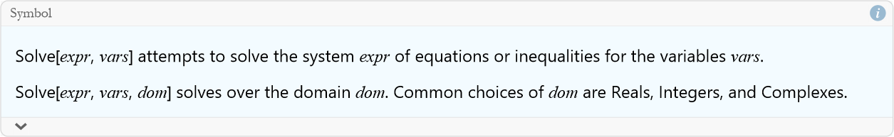
We will worry about inequalities in Lesson 9. It is important to note that WL has a slightly different language for equations than we do. We use = to signify an equation. WL uses = as an immediate assignment for a label. How do we write an equation in WL? The equation,

(6.44)

becomes

To solve this, we write,

If we want to show the solution without all the brackets, we write it as a replacement.

Solve[] does what we’ve practiced. It keeps the == balanced, isolating the variable with the same operations (addition, division) from Lesson 3, expressed algebraically in Lesson 4. It’s like having a super-smart assistant who knows Lesson 6’s method cold.

Terms and Definitions

Term/Definition 6.18 Solve[]: The Wolfram Language (WL) function that symbolically solves equations for specified variables. Basic syntax: Solve[expr, vars] attempts to solve expr for vars. It returns a list of rule-based solutions (e.g., {{x -> value}}).

Term/Definition 6.19 Equation in WL: Written using double equals == (structural equality), not single = (which is used for immediate assignment, e.g., naming an expression like eqn1 = ...).

Term/Definition 6.20 Replacement operator (/.): Used to apply solutions from Solve[] to an expression or variable, substituting the solved value(s). Example: x /. sol1 yields the value without the list-of-rules wrapper.

Term/Definition 6.21 Rule (->): WL’s arrow notation for a variable → its solution value, as returned by Solve[]. Solutions are lists of lists of rules to handle multiple solutions or systems cleanly.

Term/Definition 6.22 Domain specification: An extra argument in Solve[expr, vars, dom] to restrict solutions (e.g., Reals, Integers, Complexes). Not used in basic examples here, but mentioned in the ?Solve output.

Assumptions (the implicit beliefs the author relies on)

Assumption 6.17: The equation is solvable symbolically and has a unique solution for the requested variable. For a single linear equation a x + b == c with a ≠ 0, there is exactly one real solution. (Degenerate cases like 0 == 0 or 0 == 5 are not explored here.)

Assumption 6.18: We are working primarily over the real numbers — The basic examples imply real solutions; domain options like Reals are noted but not required for these simple cases.

Principles

Principle 6.15: Solve[] performs exactly the same balancing operations (adding/subtracting terms, dividing by the coefficient) as hand-solving linear equations, but does so instantly and without arithmetic errors.

Principle 6.16: Returning results as replacement rules (x -> value) allows clean, reusable application via /. — this is a powerful, general principle in symbolic computation that scales to systems, multiple variables, and later topics.

Exercise 6.8: Begin with Term/Definition 6.18 and copy it into your notebook. Reflect on its meaning for a few minutes. Note any thoughts that come to mind. How would you explain this to someone sitting in front of you. Write this down. Then do this for each term/definition, assumption, and principle.

Exercise 6.9: Solve these same equations for the listed unknowns using the Solve[] command:
a) 5x+2=17.
b) 3x−8=7.
c) −2x+6=10.
d) .

Systems of Linear Equations

In physics, we often encounter situations where multiple conditions must be satisfied simultaneously. Another way of saying this, is the we might need solve several equations at once. This is where systems of linear equations come into play. A system of linear equations is simply a set of two or more linear equations that share the same variables, and our goal is to find values for those variables that satisfy all the equations at the same time.

A linear equation in two variables, say x and y, looks like

(6.45)

where a, b, and c are constants. A system of linear equations is a collection of such equations. For example,

(6.46)

here, we have two equations with two unknowns, x and y. The solution to this system is a pair of values (x,y) that makes both equations true.

When solving a system of linear equations, three outcomes are possible:

Unique Solution: When this happens we say that the equations are independent and consistent, giving a single (x, y) ) pair.

No Solution: When this happens we say that the equations are inconsistent—there’s no way to satisfy them simultaneously.

Infinitely Many Solutions: This occurs when the equations are dependent, but none are what we call unique.

The Method of Substitution

When faced with a system of linear equations, we might try isolating one variable in one equation and substituting that expression into the other equation. we call this the method of substitution. It’s like solving a puzzle: you use one piece to unlock the next until the whole picture comes into focus.

The substitution method follows a straightforward series of steps:

Solve one of the equations for one variable in terms of the other.

Substitute that expression into the second equation to eliminate one variable, leaving a single equation with one unknown.

Solve the resulting equation for the remaining variable.

Plug that solution back into the expression from step 1 to find the other variable.

Check your solution in both original equations to ensure it’s correct.

Let’s walk through an example to see it in action.

Consider this system of two linear equations,

(6.47)

(6.48)

Step 1: Solve equation (6.47) for x

(6.49)

Step 2: Substitute the result from (6.49) into (6.48),

(6.50)

Step 3: Solve for y

(6.51)

Step 4: Substitute the result from (6.51) back into (6.49),

(6.52)

Step 5: Verify:

(6.53)

(6.54)

So, we now know that the solution is .

Substitution shines when one equation is easy to solve for a variable (e.g., no coefficients or simple fractions). It’s also a great mental exercise for understanding how variables relate—like tracing a thread through a physical system. However, for larger systems or equations with messy coefficients, other methods (like elimination, covered below) might save time.

The Method of Elimination

Instead of substituting, we can manipulate the equations—adding or subtracting them—to cancel out one variable, leaving us with a simpler equation to solve. This is called the method of elimination, a powerful technique for solving systems of linear equations by removing variables one at a time. This method feels like a balancing act, aligning terms to make them disappear.

The elimination method relies on the fact that if two equations are true, their sums or differences (what we might call their linear combinations) are also true. The steps are:

Adjust the equations (if needed) by multiplying them by constants so that the coefficients of one variable are equal in magnitude (and either the same or opposite in sign).

Add or subtract the equations to eliminate that variable, reducing the system to one equation with one unknown.

Solve the resulting equation.

Substitute the solution back into one of the original equations to find the other variable.

Verify the solution in both equations.

Let’s see it in practice, by considering the system,

(6.55)

(6.56)

Step 1: We want to eliminate one variable. Let’s target y. Multiply equation (6.55) by 2 and equation (6.56) by 3 to make the y-coefficients opposites (6 and -6),

(6.57)

(6.58)

Step 2: Add the equations to eliminate y,

(6.59)

Step 3: Substitute this value into (6.55),

(6.60)

Step 4: Verify,

(6.61)

This gives us the solution .

Terms and Definitions

Term/Definition 6.23 System of linear equations: A set of two or more linear equations that share the same variables. The goal is to find values of the variables that satisfy all equations simultaneously.

Term/Definition 6.24 Linear equation in two variables: An equation of the form a x + b y = c, where a, b, and c are constants or parameters (and typically a and b are not both zero).

Term/Definition 6.25 Solution to a system: An ordered pair (or tuple) (x, y, ...) that makes every equation in the system true when substituted.

Term/Definition 6.26 Unique solution: Exactly one solution exists → the system is consistent and the equations are independent.

Term/Definition 6.27 No solution: No values satisfy all equations simultaneously → the system is inconsistent.

Term/Definition 6.28 Infinitely many solutions: Any number of solutions → the equations are dependent (they represent the same relationship).

Term/Definition 6.29 Method of substitution: Solve one equation for one variable and substitute that expression into the other equation(s) to reduce the system to a single equation in one variable.

Term/Definition 6.30 Method of elimination (also called addition/subtraction method): Multiply equations by constants as needed to make the coefficients of one variable equal in magnitude (and opposite in sign), then add/subtract to eliminate that variable, reducing the system.

Term/Definition 6.31 Linear combination: Adding or subtracting (possibly scaled) equations; if the originals are true, any linear combination is also true.

Exercise 6.8: Begin with Term/Definition 6.23 and copy it into your notebook. Reflect on its meaning for a few minutes. Note any thoughts that come to mind. How would you explain this to someone sitting in front of you. Write this down. Then do this for each term/definition.

Using Solve for Systems of Linear Equations

Just as we used Solve[] for linear equations, we can use it to solve a system. If we try to solve the equation we just solved by hand we would do it this way.

Graphs

Graphs are like windows into the world of numbers—they let you see what equations are trying to tell you. I will now show you how to place points into a kind of graph. This is the groundwork for everything that follows, and in physics, it’s how we track things like an object’s position or how far it’s traveled over time. Think of it as learning to pin dots on a map—once you’ve got that, you’re ready to connect them into stories.

The Cartesian plane is a flat grid named after the mathematician René Descartes. It’s made of two number lines that cross at zero (recall the number lines we used in Lesson 3). We begin by drawing a horizontal line from left (the smaller, perhaps even negative, side) to right (the larger, perhaps positive, side). Then we place a vertical line that exactly crosses the horizontal line from the lower side to the higher side. It will look something like this.

Where they meet is often, by convention, the point where both number lines have the value 0. We call this point the origin of the Cartesian plane. Of course, you can have them meet anywhere you like, but if it’s not the origin, you need to tell people that. You can locate points on this kind of a plane by placing a dot at the relevant value of (horizontal position, vertical position). For example, (2,3) represent two units to the right, and three units up.

Exercise 6.9: Place the following points on a Cartesian plane.
1) (5,8)
2) (-4,3)
3) (-3,-3)
4) (0,4)
5) (6,0)

Plotting Points in WL

You’ve already met the Wolfram Language in Lesson 5—crunching numbers, setting variables, and even playing with some algebraic expressions. Now, let’s use it to bring our Cartesian points to life. Plotting points in WL is like telling a computer to pin your dots on the graph for you. We’ll use a command called ListPlot to do it, and since you know how WL works, you’ll catch on fast.

In WL, ListPlot is your go-to for plotting points. You give it a list of coordinates—those (x, y) pairs we’ve been placing on the Cartesian plane above—and it displays them as dots. Here’s how it works:

Write each point as {x, y} (curly braces, comma between).

Put all your points in a bigger list with {} and commas separating them.

Type: ListPlot[{{x1, y1}, {x2, y2}, {x3, y3}}].

Run that in WL, or however you are using it, and you’ll see your points pop up on a grid.

Let’s plot these points: (1, 2), (-3, 1), and (2, -4)—points you could sketch by hand

As we can see, we have three dots, no fuss. (1, 2) is right 1 and up 2, (-3, 1) is left 3 and up 1, (2, -4) is right 2 and down 4—just like on your paper graph, but now it’s digital.

Since you’ve used WL before, let’s tweak it like pros with these refinements:

Labels: Add AxesLabel -> {“x, "y"} to name the axes (note the quotes and arrow ->).

Bigger Dots: Use PlotStyle -> PointSize[0.02] to make points stand out (0.02 is a nice size).

Write this:

Result: Easily visible dots with labeled axes.

Graphs

Exercise 6.10: Place the following points on a Cartesian plane.
1) (5,8)
2) (-4,3)
3) (-3,-3)
4) (0,4)
5) (6,0)

Plotting Points in WL

Write each point as {x, y} (curly braces, comma between).

Put all your points in a bigger list with {} and commas separating them.

Type: ListPlot[{{x1, y1}, {x2, y2}, {x3, y3}}].

Run that in WL, or however you are using it, and you’ll see your points pop up on a grid.

Let’s plot these points: (1, 2), (-3, 1), and (2, -4)—points you could sketch by hand

As we can see, we have three dots, no fuss. (1, 2) is right 1 and up 2, (-3, 1) is left 3 and up 1, (2, -4) is right 2 and down 4—just like on your paper graph, but now it’s digital.

Since you’ve used WL before, let’s tweak it like pros with these refinements:

Labels: Add AxesLabel -> {“x, "y"} to name the axes (note the quotes and arrow ->).

Bigger Dots: Use PlotStyle -> PointSize[0.02] to make points stand out (0.02 is a nice size).

Write this:

Result: Easily visible dots with labeled axes.

Terms and Definitions

Term/Definition 6.32 Graph (or Cartesian plane): A flat grid formed by two perpendicular number lines crossing at zero (the origin), used to plot points and visualize relationships.

Term/Definition 6.33 Origin: The point (0, 0) where the horizontal and vertical axes intersect.

Term/Definition 6.34 Axes (plural of axis): The horizontal (often called thex-axis) and vertical (often called they-axis) number lines forming the Cartesian plane.

Term/Definition 6.35 Point (on graph): A location specified by an ordered pair (x, y), where x is horizontal position and y is vertical position.

Term/Definition 6.36 ListPlot: A Wolfram Language command that plots a list of coordinate pairs as points on a Cartesian plane (e.g., ListPlot[{{x1,y1}, {x2,y2}, ...}]).

Term/Definition 6.37 AxesLabel: An option in plotting functions to label the axes (e.g., AxesLabel → {"x", "y"}).

Term/Definition 6.38 PlotStyle: A WL option to customize appearance (e.g., PlotStyle → PointSize[0.02] for larger dots).

Term/Definition 6.39 PointSize: A WL plotting directive to set the size of plotted points (e.g., 0.02 for visible dots).

Assumptions (the implicit beliefs the author relies on)

Assumption 6.19: The origin (0, 0) is the reference point where axes cross.

Assumption 6.20: Positive directions are right (x) and up (y) by convention.

Assumption 6.21: Manual sketching and computational plotting complement each other for learning.

Principles

Principle 6.17: Practice plotting by hand first, then verify/complement with WL.

Exercise 6.11: Begin with Term/Definition 6.32 and copy it into your notebook. Reflect on its meaning for a few minutes. Note any thoughts that come to mind. How would you explain this to someone sitting in front of you. Write this down. Then do this for each term/definition, assumption, and principle.

Plotting Equations by Hand

You’ve mastered pinning individual points on the Cartesian plane—now let’s see what happens when you plot a whole equation. A linear equation like y = 2x + 1 isn’t just one point—it’s a rule that generates lots of them. By plotting a few and connecting the dots, you’ll uncover a segment of a straight line—the signature of “linear” in action.

Step 1: Pick Your Horizontal Values
Start with your equation—say, y = 2x + 1. To plot it, choose a few x values (the horizontal axis). Simple numbers like -1, 0, and 1 work well because they’re easy to calculate and spread across the origin:

You can pick more, but three’s a good start to spot the pattern.

Step 2: Calculate the y Values
Plug each x into the equation to find the matching y (vertical axis).

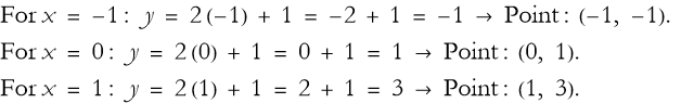
Now you’ve got three points: (-1, -1), (0, 1), and (1, 3).

Step 3: Plot the Points
On your graph paper, mark these points:

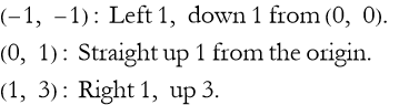
Put a dot at each spot. These are like snapshots of where the equation lives on the plane.

Step 4: Connect the Dots
Here’s the magic: take a ruler and draw a straight line through all three points. If you’ve done it right, they’ll line up perfectly. Why? Because y = 2x + 1 is a linear equation—it makes points that form a straight line. Extend the line past your points in both directions (arrows at the ends show it keeps going). That’s the full picture of the equation!

Plotting Equations in WL

You’ve already used ListPlot to pin points in the Wolfram Language and connected them by hand to see lines. Now, let’s level up—WL can draw those lines for you with a single command called Plot. Instead of picking points one by one, you’ll tell WL the equation—like y = 2x + 1—and it’ll graph the whole thing instantly.

The Plot command draws the full line of an equation over a range of x values (or whatever variable you want to use). Here’s the setup:

Replace “equation” with your formula (e.g., 2 x + 1), and set the x range (e.g., {x, -2, 2} for x from -2 to 2).
Run it in WL, and you’ll see a smooth line—no dots to connect!

Let’s plot y = 2x + 1.

As an exercise, invent linear equations and try this out on them. (Hint: just copy the code and change the expression).

You can apply multiple equations by making a list of equations. For example

Assumptions(the implicit beliefs the author relies on)

Assumption 6.22: Linear equations produce straight lines when plotted.

Assumption 6.23: Plotting a few points and connecting them reveals the full line for linear equations.

Assumption 6.24: Simple values (e.g., -1, 0, 1) are sufficient to spot the pattern in linear equations.

Assumption 6.25: Axes labels and point size customization improve clarity and readability of plots.

Principles

Principle 6.18: Graphs turn equations into visual stories: plot points or functions to see patterns (e.g., straight line for linear equations).

Principle 6.19: Plot multiple equations together: Plot[{expr1, expr2, ...}, {x, xmin, xmax}].

Principle 6.20: Verify plots: hand-sketch first, then compare with WL output.

Principle 6.21: Graphs reveal linearity (straight lines) and relationships in physics (motion, forces, etc.).

Exercise 6.12: Begin with Assumption 6.22 and copy it into your notebook. Reflect on its meaning for a few minutes. Note any thoughts that come to mind. How would you explain this to someone sitting in front of you. Write this down. Then do this for each assumption, and principle.

Summary

Write a summary of this lesson as an exercise.

For Further Study

I. M. Gelfand, A. Shen, (1993), Algebra, Birkhauser. As stated in Lesson 4a, I can think of few that are better.

Navy Education and Training Professional Development and Technology Center, (1980) Mathematics, Basic Math and Algebra, NAVEDTRA 144139, Reprinted in 1985 (available for free at the Internet Archive https://archive.org/details/US_Navy_Training_Course_-_Mathematics_Basic_Math_and_Algebra). This is the first of a comprehensive set of manuals for training sailors in basic math.

Created with the Wolfram Language