Lesson 5: Introduction to the Wolfram Language

“Computation is destined to be the defining idea of our future, and the Wolfram Language is the tool to make that happen.” Stephen Wolfram

“The best way to learn mathematics is to use it in the service of some great purpose.” George Boole

Introduction

Welcome to a new frontier in our journey through theoretical physics—we present a tool that bridges the abstract beauty of mathematics (a thing we might not have seen, yet) with the tangible wonders of the physical world: the Wolfram Language. Developed by Stephen Wolfram and his team at Wolfram Research. This computational language empowers us to explore, simulate, and solve problems in ways that once required teams of experts or rooms full of machinery. For the amateur physicist, it’s a gateway to performing complex calculations, visualizing phenomena, and experimenting with ideas without needing advanced programming skills. In this chapter, we’ll embark on a hands-on introduction to the Wolfram Language, starting with its basic syntax and structure, then moving into how it can represent and manipulate the mathematical expressions we’ve encountered so far—think numbers, expressions, and polynomials brought to life. We will discuss different versions of it, and even some free alternatives. No prior coding experience is assumed; our goal is to equip you with a tool that amplifies your curiosity, and builds on pencil and paper. By chapter’s end, you’ll see how the Wolfram Language isn’t just a calculator—it’s a playground for discovery, setting the stage for deeper explorations in our series.

Using Computers in Physics

Computers are electronic devices that are capable of acquiring, storing, and manipulating data far faster and, often, more accurately than the human mind alone. You can think of it as a tireless assistant for the physicist, capable of performing calculations in mere seconds that once took hours, and even days, by hand. Of course, we must always verify these results where possible—double-checking with simple hand calculations or known values—because even the smartest machine can misstep if given flawed input or instructions.

The first electronic computer of this type was made in the mid to late 1940s to assist in calculations required for the development of the hydrogen bomb. Since then, computers have become an integral part of daily life. With modern computers you can collect data from instruments and experiments and store it in files, you can analyze the data, you can construct predictive models, display the data and the predictions, you can write up the results and present them in web pages, journals, and live presentations.

Broadly speaking, a computer consists of a central processing unit (CPU) that controls everything, a memory unit that stores information for active use by the CPU, peripheral devices for display, long-term storage, printing, and communication with other computers, and the computer will also have one or more internal circuits for connecting all of the elements of the computer together—what we call a bus. We communicate with a computer through a keyboard and a display monitor, and we often use a mouse or a track ball.

In order to make a calculation that operates on a computer you must be able to write out a complete list of instructions telling the computer what to do. Such a list of instructions is called an algorithm. Computers all have a language that is unique to their CPU called a machine language. Few people communicate directly with the computer in machine language these days. Most algorithms can be converted to machine language from some other programming language through some kind of interface. Such interfaces use either active conversion as you write each instruction (this kind of language interface is called an interpreter), or the algorithm is written in its entirety and then converted all at once to machine language (this is called a compiler). The process of translating an algorithm into a computer language is called coding. A translated algorithm is called a computer code or program. Often a computer language will have a special program that contains a place where code is written, other places where information about the language is stored for reference, and there can even be tools to assist in writing your code; such a program is called a programming environment.

To operate, or run, a program the first instruction of the program is directed from long-term storage to the CPU and it acts on any relevant data that is kept in long-term storage for this purpose. Once this is completed the results are placed in memory. The CPU is then directed to the next instruction and the process is repeated. This continues until every instruction has been completed.

Terms and Definitions

Term/Definition 5.1 Computer: An electronic device capable of acquiring, storing, and manipulating data quickly and accurately.

Term/Definition 5.2 Central Processing Unit (CPU): The component that controls the computer’s operations and executes instructions.

Term/Definition 5.3 Memory unit: The component that stores information for active use by the CPU.

Term/Definition 5.4 Peripheral devices: External devices for input/output (e.g., display, storage, printing, communication).

Term/Definition 5.5 Bus: Internal circuits connecting all computer components.

Term/Definition 5.6 Algorithm: A complete list of instructions telling the computer what to do.

Term/Definition 5.7 Machine language: The low-level language unique to a computer’s CPU.

Term/Definition 5.8 Interpreter: An interface that converts algorithm instructions to machine language actively (line-by-line as written).

Term/Definition 5.9 Compiler: An interface that converts an entire algorithm to machine language all at once.

Term/Definition 5.10 Coding: The process of translating an algorithm into a computer language.

Term/Definition 5.11 Computer code (or program): A translated algorithm in machine language.

Term/Definition 5.12 Programming environment: A special program with areas for writing code, language reference, and tools to assist coding.

Assumptions (the implicit beliefs the author relies on)

Assumption 5.1: Computers vastly outperform humans in speed and accuracy for repetitive calculations.

Assumption 5.2: Computer results must always be verified (due to possible input/instruction errors).

Assumption 5.3: Modern computers are essential tools for data collection, analysis, modeling, visualization, and presentation in physics.

Assumption 5.4: Basic computer architecture (CPU, memory, peripherals, bus) is consistent across systems.

Assumption 5.5: Human-computer interaction primarily uses keyboard, monitor, mouse/trackball.

Assumption 5.6: Machine language is too low-level for most users; higher-level languages with interpreters/compilers are standard.

Assumption 5.7: Programs execute sequentially: fetch instruction, act on data, store results, proceed to next.

Exercise 5.1: Begin with Term/Definition 5.1 and copy it into your notebook. Reflect on its meaning for a few minutes. Note any thoughts that come to mind. How would you explain this to someone sitting in front of you. Write this down. Then do this for each term/definition, and assumption.

The Wolfram Language

Imagine a tool that combines the precision of mathematics, the power of computation, and the curiosity of a physicist into a single, accessible language—this is the Wolfram Language (WL). It’s a high-level programming language—this means it takes commands and converts them into machine language. WL is designed to make complicated calculations as intuitive as writing a sentence. Unlike traditional programming languages that often demand intricate coding skills, WL is built with a vast library of built-in functions and knowledge, allowing even beginners to tackle sophisticated problems with just a few lines of code. For the amateur physicist, it’s a revelation; a way to explore concepts without getting bogged down in endless manual computations or advanced software engineering. In this chapter, we’ll dive into its basics—how to write expressions and perform operations—using the free Wolfram Engine or Mathematica if you have it. The Wolfram Language isn’t just about getting answers; it’s about asking questions, testing ideas, and seeing your work come alive. As we proceed, always remember to verify your computer’s outputs where possible, grounding its power in the reality we aim to understand

Mathematica

Mathematica (MMA) is a programming environment that uses the Wolfram Language (WL) as its computer language. The place where coding takes place is most often in a place called a notebook. The notebook is often an interpreter, though WL has a compiler that is becoming integrated into more and more functions with every new version release, allowing you to compile complicated instructions so that they run faster. Thus MMA can be thought of as a hybrid interpreter/compiler.

There are hundreds of computer languages and dozens of programming environments—many of them are free. This being the case, why choose Mathematica? MMA has many useful aspects that are not individually unique to it, but are collectively unique. MMA/WL is platform independent (it does not depend on which operating system or CPU you use). It allows you to create programs based on algorithmic procedures (called procedural programming and this style of programming is familiar to everyone who has programmed in C, C++, Java, Python, etc.), WL also allows you to manipulate combinations of instructions (what we call functional programming), it allows you to rewrite instructions by applying rules (what we could call rule-based or transformational programming), and you can mix and match these kinds of programming as you like. You can create reports and finished papers (this lesson is written entirely in Mathematica, for example), you can import and export data, you can perform calculations that are entirely symbolic, you can perform calculations that are entirely numerical, and you can perform calculations that are both symbolic and numerical. There is no other system that has all of these capabilities that are free.

The professional/academic version of Mathematica is available from Wolfram Research and it allows you to produce code and sell it, to write technical documents (such as this lesson) and sell them, or to provide consulting services for pay. There is a version that is entirely in a cloud that you can log into over the Internet. There is a reduced price version for hobbyists, the caveat is that you cannot use this version for making money. There is also a version for use by students with a valid student ID. Finally, you can purchase a Raspberry Pi computer, and they already have Mathematica. All of these versions of Mathematica are the same in terms of functionality. There is even a freely available version, called The Wolfram Engine that uses a command line interface (CLI),  we will see more about this below.

There are some oft-repeated statements made about MMA/WL that are not true. Many people choose not to use MMA because it is slow compared to some other language. It might be true that optimized code in a special language might be a few percent faster than MMA, but there are two things that need to be pointed out. If you convert directly from, say, a procedural language to procedural code in MMA it is not the most efficient use of MMA. It is better to choose what parts of MMA are best for the algorithm you want to code (perhaps even changing the algorithm). The other thing to consider is development time, MMA requires only a fraction of the time to code as other languages. If you optimize the implementation of an algorithm in MMA/WL it will run competitively.

Another complaint is that MMA is a black box, where you have no idea what is going on once you start using a built-in function. It is true that some functions in WL or MMA are so complicated and huge that the specific method being used is not easy to follow. There is a continual struggle to document functions and methods that often lags behind development. On the other hand you are not restricted to use built-in functions. If you are uncertain about how something is being done, write your own code. Compare it with the built-in function.

Another complaint is that MMA/WL can only handle small projects on a desktop computer. That is sheer nonsense. Wolfram|Alpha is an online interactive system maintained on a large cluster of computers accessible to anyone over the Internet and consists of millions of lines of MMA/WL code alongside C++ code.

Terms and Definitions

Term/Definition 5.13 Wolfram Language (WL): A high-level programming language designed for intuitive mathematical and computational tasks, with vast built-in functions and knowledge.

Term/Definition 5.14 Mathematica (MMA): A programming environment that uses the Wolfram Language as its language; primarily notebook-based.

Term/Definition 5.15 Notebook: The main interface in Mathematica for writing, executing, and documenting code (often an interpreter).

Term/Definition 5.16 Interpreter: A system that converts and executes code line-by-line (MMA notebooks often function this way).

Term/Definition 5.17 Compiler: A system that converts entire code to machine language at once for faster execution (WL increasingly integrates compilation).

Term/Definition 5.18 Procedural programming: Programming style using algorithmic steps/procedures (familiar from C, Java, Python).

Term/Definition 5.19 Functional programming: Programming style manipulating combinations of instructions/functions.

Term/Definition 5.20 Rule-based (or transformational) programming: Programming style rewriting instructions by applying rules.

Term/Definition 5.21 Wolfram Engine: A free version of WL using a command-line interface (CLI).

Term/Definition 5.22 Cloud version: Mathematica accessible over the Internet.

Term/Definition 5.23 Black box: Criticism that some built-in functions hide internal workings (partially true for complicated functions).

Assumptions (the implicit beliefs the author relies on)

Assumption 5.8: Wolfram Language/Mathematica is uniquely powerful due to its combination of features (platform independence, multiple programming paradigms, symbolic/numeric capabilities, documentation tools).

Assumption 5.9: No other free system matches MMA/WL’s collective capabilities.

Assumption 5.10: Development time in WL is significantly shorter than in other languages, offsetting potential speed differences.

Assumption 5.11: Users can always write custom code to avoid “black box” issues.

Assumption 5.12: Verifying computer outputs against hand calculations/known values is necessary.

Principles

Principle 5.1: MMA notebooks are ideal for interactive coding, documentation, and reporting.

Principle 5.2: Optimize algorithms for WL strengths rather than direct translation from other languages.

Exercise 5.2: Begin with Term/Definition 5.13 and copy it into your notebook. Reflect on its meaning for a few minutes. Note any thoughts that come to mind. How would you explain this to someone sitting in front of you. Write this down. Then do this for each term/definition, assumption, and principle.

What is a Computer Algebra System (CAS)?

This is a now, mostly, outdated term to describe systems that allow you to perform symbolic mathematical operations on a computer instead of the tradition numerical operations. I consider it outdated because neither of the two principal systems (Mathematica and Maple) are strictly algebra systems, as they both have very robust numerical and general programming capabilities.

The first CAS I know of was called MathLab and came out in 1964. It brought about what can be considered the first generation of CAS. These are exclusively written in, and require the use of, the programming language LISP. Reduce came out in 1968, it is now in the public domain. Reduce is also a first-generation system—it is written in, and requires, LISP. It is freely available from the website: http://www.reduce-algebra.com/ . Then Macsyma was developed in 1969. This had an interesting development path. Macsyma was sold commercially for a while, and is now defunct. MIT had a version of it under the DOE, called Maxima, which entered the public domain. This is now available at the website: http://maxima.sourceforge.net/ . Scratchpad was the next first-generation system and it came out in 1974. This was a remarkable system that later became Axiom. Axiom is now terribly out of date, at least in terms of its interface, and is available at the web site: http://axiom.axiom-developer.org/ . MuMath, which later became Derive, came into being in 1979, and was the last of the first-generation systems developed in LISP. Derive had an interesting life. Starting out as a reduced-strength CAS for students, it saw life in certain powerful hand-held calculators.

SMP (Symbolic Manipulation Program) was pretty revolutionary for its time, it was developed by Chris Cole and Stephen Wolfram in 1981 while they were at Caltech. Maple is a second-generation system written in C and C++ and first arrived in 1983 from Waterloo Software (now owned by Cybernet Systems Group). It is now a fully capable environment for programming and scientific discovery.

Mathematica came out in 1988, also written in C/C++. Depending on who you talk to, it is the most popular of the general CAS. When Stephen Wolfram left Caltech he was unable to take SMP with him, as it was being sold by a different company. Wolfram, along with other developers produced the first commercial version of MMA in 1988 where it had approximately 500 functions. Each new version added new functions where the newest version has more than 6000 built-in functions. Of course, it has always had a programming language that in 2013 was officially named the Wolfram Language (WL). So, if it doesn’t do something you want it to do, you can program a new function or even a large software system.

MuPAD came out in 1992 and is available only as a MATLAB add-on. I consider this to be extremely expensive, since you need MATLAB and then MuPAD.

The Structure of Mathematica

When you start Mathematica it loads into memory from long-term storage. The link to the CPU is called the Mathematica Kernel. It also loads a user interface file called the Notebook Front End, or just the notebook. Multiple notebooks can be loaded at once. Notebooks can be saved into long-term storage once you name them. You can load special programs that extend the capabilities of the kernel, these are called packages.

Most of the work done in Mathematica takes place in the notebook. This front end interface easily allows you to write programs, include text, graphics, and even sound into one place. An important aspect of notebooks are the brackets that appear on the far right side, these are called cells. All instructions appear in cells. A cell encompasses a paragraph. They are the basic element of a notebook. You can copy and paste cells, you can change their format, and you can execute any instructions contained in such a cell. In Windows you place the cursor anywhere in the instruction you want to execute, or you highlight the cell (by clicking on it), and then you hold down the Shift key and press Enter.

If you have a multiprocessor computer, then you can have a number of kernels running in parallel, one on each of a number of processors (usually half the number of processors you have on your computer). If you have a network of computers, and each computer has MMA, then you can connect them over a local-area network (LAN) by using the built-in Lightweight Grid. This allows you to have different processes operating on multiple cores on multiple computers.

The fundamental object that is placed in active memory is called an expression. Everything you work on in a cell is an expression, whether it is a calculation, a paragraph of text, an image, a sound file, a video, or any combination. MMA/WL has a sophisticated system for interpreting expressions. Say we have the expression a+b. This is an expression made up of three sub-objects that we can call tokens. There are two symbolic tokens, a and b, and one operator token +. MMA/WL looks at the expression and sees the operator first in the form of a header, Plus, then the symbols, so it sees Plus[a,b]. Simple expressions can be used to build more complicated expressions.

New functions can be created in notebooks. Sometimes, especially with large collections of functions we might place them all into a special notebook that we call a package. A package is stored in a folder called AddOns and as you might expect they are loaded to add new functionality to MMA/WL.

The Notebook Front-End

When you step into the Wolfram Language, your playground is the Notebook—a dynamic, interactive interface that brings computation to life in a way that’s both intuitive and powerful. Think of the Notebook as a digital workspace where you can write commands, see instant results, and weave together text and expressions all in one place. Available through the Wolfram Research as either the stand-alone Wolfram Player or built-in to the Mathematica software, this front-end transforms your screen into a canvas for exploration, letting you type a line like,

and instantly compute it with a press of a key. Each Notebook is a living document, where you enter code in cells (the small brackets on the right-hand side), execute it, and watch outputs appear below, all while adding notes or headings to keep your thoughts organized. For the amateur physicist, this is a game-changer—gone are the days of juggling calculators and graph paper; here, you can experiment with expressions in real time, tweaking variables and seeing the output adjust before your eyes. The Notebook’s strength lies in its flexibility: it supports trial and error, lets you revisit and refine ideas, and even saves your work for later. As you use it, always take a moment to verify your results—cross-check with simple calculations or known results—to ensure the magic on-screen matches the reality we’re studying.

Terms and Definitions

Term/Definition 5.24 Computer Algebra System (CAS): A system for performing symbolic mathematical operations on a computer (as opposed to purely numerical); now somewhat outdated term since modern systems (Mathematica, Maple) include robust numerical and general programming capabilities.

Term/Definition 5.25 Mathematica Kernel: The core computational engine of Mathematica that loads into memory and performs calculations.

Term/Definition 5.26 Notebook Front End (or notebook): The user interface in Mathematica for writing, executing, and documenting code; dynamic and interactive.

Term/Definition 5.27 Cell: The basic unit in a notebook (bracketed on the right); encompasses a paragraph or block of input/output.

Term/Definition 5.28 Package: A special notebook/file containing collections of functions to extend Mathematica's capabilities; loaded from AddOns folder.

Term/Definition 5.29 Lightweight Grid: Built-in Mathematica feature for parallel computation across multiple cores or networked computers.

Term/Definition 5.30 Expression: The fundamental object in Mathematica; everything (calculations, text, graphics, sound, etc.) is represented as an expression.

Term/Definition 5.31 Token: Sub-objects within an expression (e.g., symbols a, b and operator + in a + b).

Assumptions (the implicit beliefs the author relies on)

Assumption 5.13: Historical first-generation CAS (1960s–1970s) were LISP-based and limited.

Assumption 5.14: Modern CAS like Mathematica (1988 onward) are general-purpose computational environments.

Assumption 5.15: Wolfram Language (named 2013) is the underlying language of Mathematica.

Assumption 5.16: Users can extend functionality via custom functions or packages.

Assumption 5.17: Parallel/grid computing is accessible even on desktop/multi-computer setups.

Principles

Principle 5.3: Mathematica structure: Kernel (computation) + Notebook Front End (interface) + optional packages.

Exercise 5.3: Begin with Term/Definition 5.24 and copy it into your notebook. Reflect on its meaning for a few minutes. Note any thoughts that come to mind. How would you explain this to someone sitting in front of you. Write this down. Then do this for each term/definition, assumption, and principle.

Acquiring the Wolfram Engine

Even the hobby version of MMA costs money. If your budget is so tight you cannot afford Mathematica, or you want to play with it to see if it is what you want, you can try the free version. This allows you to dive into the Wolfram Language and play around with its computational power. The Wolfram Engine is the heart of the system that executes your commands. Fortunately, acquiring it is straightforward and free for non-commercial use, making it an ideal starting point for amateurs like us. Begin by visiting the Wolfram website (www.wolfram.com/engine) and selecting the “Free Wolfram Engine for Developers” option. You’ll need a Wolfram ID—create one with an email address if you don’t have it already—then download the installer for your operating system (Windows, Mac, or Linux). The process is simple: run the installer, follow the prompts, and activate the engine with your Wolfram ID credentials. This free version, known as the Wolfram Engine Community Edition, is perfect for personal exploration, education, or pre-production projects, though it restricts commercial use without a paid license. Once installed, you can access it via a command-line interface or connect it to tools like Jupyter notebooks or the Wolfram Development Platform for a more visual experience. After setup, test it with a basic command—like calculating the speed after two seconds of gravitational acceleration (falling),

and verify the result (19.6 meters per second) by hand to ensure it’s working correctly. This step confirms your tool is ready.

Using WolframScript

Once you’ve acquired the Wolfram Engine, WolframScript offers a nimble way to tap into its power without needing a full graphical interface—just a simple command line on your computer. Think of WolframScript as a direct line to the Wolfram Language, letting you type commands and get answers instantly, perfect for quick calculations. To start, ensure the Wolfram Engine is installed (as outlined above), then open your computer’s terminal—Command Prompt on Windows, Terminal on Mac or Linux—and type wolframscript. If installed correctly, you’ll see a prompt where you can enter commands like 2 * 9.81 to calculate the speed of a falling object after 2 seconds (output: 19.62). For more control, write a script file—say, physics.wls—with commands like Print[Force = 5 * 3] to compute force (15 units of force), save it, and run it with wolframscript -file physics.wls. This method works for repetitive tasks or sharing calculations, and you can even automate problems from the command line. Its lightweight nature suits amateurs who want results fast without a steep learning curve.

Using a Text Editor

For those of us diving into the free alternative to the Wolfram Language, a text editor can transform how we write, test, and refine our computational ideas, offering a step up from the command-line simplicity of WolframScript. A text editor is a program where you can craft scripts—sets of code—saved as files to run later, giving you the freedom to experiment at your own pace. One standout example is Jupyter Notebook, a free, open-source tool that blends coding with a notebook-style interface, perfect for amateurs who want to mix Wolfram Language commands with notes and visuals. To use Jupyter with the Wolfram Engine, first install Jupyter (via Python’s pip install jupyter in your terminal), then add the Wolfram Language kernel by following Wolfram’s setup guide (available at wolfram.com). Open Jupyter by typing jupyter notebook in your terminal, and create a new notebook with the Wolfram Language kernel. Here, you can type a command like N[9.81 * 2] in a cell to compute a falling object’s speed after 2 seconds (19.62), hit Shift+Enter to run it, and see the result.

Terms and Definitions

Term/Definition 5.32 Wolfram Engine: The free core computational component of the Wolfram system that executes Wolfram Language commands (Community Edition for non-commercial use).

Term/Definition 5.33 Wolfram ID: An account required for activating the Wolfram Engine (created with an email address).

Term/Definition 5.34 WolframScript: A command-line tool for running Wolfram Language scripts directly from the terminal.

Term/Definition 5.35 Script file: A saved file (e.g., .wls extension) containing Wolfram Language commands to be executed via WolframScript.

Term/Definition 5.36 Text editor (in context): A program for writing and editing code/scripts (e.g., for Wolfram Language).

Term/Definition 5.37 Jupyter Notebook: A free, open-source interactive notebook environment that supports mixing code, text, and visuals; can be connected to the Wolfram Engine.

Term/Definition 5.38 Kernel (Wolfram Language kernel in Jupyter): The backend that executes Wolfram Language code within Jupyter.

Assumptions (the implicit beliefs the author relies on)

Assumption 5.18: Budget constraints may limit access to full Mathematica; free alternatives suffice for learning/exploration.

Exercise 5.4: Begin with Term/Definition 5.32 and copy it into your notebook. Reflect on its meaning for a few minutes. Note any thoughts that come to mind. How would you explain this to someone sitting in front of you. Write this down. Then do this for each term/definition, and assumption.

Exercise 5.5: If you do not get Mathematica, then go ahead and get the free Wolfram Engine.

Arithmetic Operations in WL

Mathematica allows you to perform each arithmetic operation and its inverse. To add two numbers, say 454 and 63, we open an Input Cell and write

Exercise 5.6: Add any two numbers using Mathematica. Type list1, then =, this will immediately assign whatever follows to the name list1. You can make a list by writing a curly bracket, {, and then listing each number with a comma separating each, and then closing the list with the end curly bracket, }.  Execute this command, placing list1 into active memory. Type ?Total to get the write-up of the command Total. In a new line write Total[list1] in order to get the sum of all the elements of your list.

To multiply two numbers, say 64 and 5155158, we can write

or we just put a space between the factors,

Note that MMA fills in a multiplication symbol when applying the space to numbers.

Exercise 5.7: Multiply any two numbers.

We can raise a number, say, 55 to a power, say 8,

we can also type 55 and then the command Ctrl 6 and then 8.

Exercise 5.8: Raise any number to some power.

We can take the inverse of addition, subtraction, by writing

Exercise 5.9: Subtract any number by some number.

The inverse of multiplication is, of course, division,

Exercise 5.10: Divide any number by some number.

The first inverse of raising a number to a power is to take the power-order root (the surd) of the exponent to get the base. Here we use the command Surd, followed by square brackets [], the square bracket is standard notation for the arguments of a built-in function.

we can also write this using a fractional power.

Exercise 5.11: Find the Surd of any number to some fractional power.

The second inverse of raising a number to a power is to take the base logarithm of the exponent to get the power, here the base is 55.

Exercise 5.12: Find the logarithm of any number to some number base.

Let’s say we wanted to find the 9th root of our exponent,

This is an exact result, and it is very difficult to interpret it. It would be better if we could get a numerical approximation of this, we can take the previous expression and wrap an N[] around it to get a floating-point approximation.

Or we can write //N after the expression.

Or we can specify that we want the surd out to as many as ten decimal places

of course it doesn’t give more digits than are needed.

Exercise 5.13: For previous answers that were difficult to interpret, find the numerical approximation to some number of digits of precision.

Algebraic Expressions in WL

As stated above, we are not restricted to numerical calculations. When doing symbolic calculations it is a good idea to assign a name to each expression as you enter it. We will use the immediate assignment symbol = to assign an expression to our label. Here we invent three expressions. Each is separated by the semicolon, ;, in MMA this tells the system to suppress the output.

Exercise 5.14: Create an algebraic expression and assign it the label of ex1.

We can add expressions.

We can subtract expressions.

We can multiply expressions.

We use the Expand[] command.

We can apply a function like Expand, by writing our expression then including a double slash at the end, and then write Expand.

We can divide expressions. If you want to make a rational expression type in the numerator then hold down the [CTRL] key and press the forward slash key.

We can take a power

We can find a root. Here we use the Simplify function to reduce exp8 into its simplest form.

Here we see MMA getting confused. We might need to rewrite this to an equivalent expression. We can impose Rule 4.9 and Rule 4.4.

Exercise 5.15: Raise your created expression to some power, label this ex2.

Simplify[]

As we have seen above, the Simplify[] function is like a trusty assistant that tidies up messy algebraic expressions, making them easier to read and use—an invaluable skill when juggling the equations of physics. Simplify[] takes an expression and reduces it to its simplest form by combining like terms, canceling common factors, or applying basic algebraic rules—all with a single command. For example, suppose you’re summing forces on an object: enter Simplify[2x + 3x - x + 5] in a Notebook or WolframScript, and WL returns 5x + 5, neatly combining the x terms. For a physics twist, consider gravitational potential energy near Earth’s surface, ; type

factoring out variables and dropping zero terms. Even rational expressions shine—try this,

As you can see, this function saves time and reduces errors.

Exercise 5.16: You have determined that the speed given an acceleration a and a quantity of units of time (t) is given as s = a t. You then calculate the kinetic energy to be, . Use Simplify[] to reduce this to it s simplest form.

We often encounter expressions that look intimidating—long chains of terms or nested fractions as examples. The WL provides a powerful tool to tame these beasts: the FullSimplify command. This function goes beyond basic simplification (like what Simplify offers) by applying a wider range of mathematical transformations and identities to produce the most compact and elegant form of an expression possible.

Let’s start with a simple example. Suppose you’re working with an expression like this:

You notice WL only returned the expression. Let’s try Simplify.

We should be a bit suspicious  of this. Why? We have no reason to believe that this is as simple as it can be. All Simplify did was apply a GCF and then simplify the numerator. Now, it is possible that is as far as it goes. We might try applying it again.

No change in the result. Now we try FullSimplify.

What happened here? FullSimplify performed a polynomial factorization and gave us the simplified expression. So, why not use it all the time? It’s computationally intensive because it tries every trick in the book—factoring, applying identities, reducing fractions, and more. For quick, basic cleanup, Simplify might suffice. But when you’re stuck with a complicated expression and need the most concise form (or suspect a hidden physical insight), FullSimplify is your ally.

You can also guide FullSimplify with assumptions to tailor its output. For instance, if you’re working with a positive variable (common in physical quantities like mass or time), try,

Why doesn’t MMA evaluate this? It does not know what values of x we are using. It is giving the most general answer. If x is negative the answer is different than if x is positive or 0. How do we write that? We say that x is more than 0, or x > 0. Try this:

The arrow is made by typing - followed by >, MMA immediately turns that into the arrow. What about this:

In physics, such assumptions often align with the problem’s context, making your results more meaningful.

Expand[]

In physics, we often start with compact mathematical expressions that hide their full detail. The WL can handle that with the Expand[] command. Unlike Simplify and FullSimplify, which condense expressions into their most elegant form, Expand[] does the opposite: it multiplies out factors and distributes operations, giving you the raw, fully expanded version of an expression.

Let’s start with a basic example. Suppose you’re working with a binomial squared, like

We can expand this using the Expand[] command.

We can see that Expand applied the FOIL method to give us , this can be called the binomial theorem, where theorem is a name given to rules that have been mathematically proven, a thing we will learn how to do in Lesson 11. This is handy when you need to see all of the components.

Now, consider a physics-inspired case, like the square of a speed sum, this quantity tells us how fast the object is going after so much time goes by,

(5.1)

To write a subscript in MMA, hold down the [CTRL] key and then type -,

This expanded form might be the starting point for calculating kinetic energy.

The Expand[] command shines when dealing with products of polynomials. Imagine a force expression multiplied by a displacement (the distance traveled), such as

Here, it distributes each term, then combines like terms into the answer given.

Expand[] works on products, not ratios, and won’t simplify unless you pair it with other commands. Expand[] doesn’t cancel or simplify—it assumes you want the full picture. If you need to expand only part of an expression or handle fractions, combine it with commands like Numerator[] or follow up with Simplify[]. For instance:

Note that expr18 is different than expr19.

In short, Expand[] is your go-to for unpacking the mathematics of physics into its bare bones. It’s less about elegance and more about clarity—perfect when you’re dissecting a problem step-by-step.

Exercise 5.17: The speed of an object has the form , use Expand to write it out fully.

Exercise 5.18: An object experiencing a gravitational force is displaced by . Use Expand to see each term explicitly.

Exercise 5.19: A specific spring force is found to depend on two factors (k x +1)(x-2). Use Expand to see how the factors combine. Can you interpret the cross terms (the inside and outside terms).

Factor[]

In physics, expressions often arrive as sprawling sums—think of a polynomial describing energy or motion. The WL Factor[] command helps you reverse-engineer these, pulling out common factors and rewriting them as products. It’s the flip side of Expand[], which multiplies everything out, and a cousin to Simplify and FullSimplify, which seeks the sleekest form. With Factor[], you’re looking to spot structure, making expressions easier to interpret or solve.

Let’s start simple. Suppose you’re analyzing a position expression

(5.2)

We can use Factor[].

Let’s say we have a kinetic energy expression

(5.3)

We can use Factor[] to get the following result.

So we have a perfect square.

Factor[] handles bigger polynomials too. For example,

(5.4)

We can apply Factor.

Exercise 5.20: Factor .

Exercise 5.21: An energy expression reduces to . Use Factor[] to break it down.

Exercise 5.22: A spring has an energy expression of . Use Factor[] on it and try to explain the common factor.

Problem 5.23: Begin by using Factor on . What happens when you then Simply the result? How do you return the original expression?

Collect[]

When you’re knee-deep in a physics calculation, the result can be a jumble of terms. The WL Collect[] command helps you tidy up by grouping terms around a chosen variable, making patterns pop out. It’s less about simplifying (like Simplify or FullSimplify) or factoring (like Factor[]) and more about organizing. Think of it as a middle ground between Expand[]’s sprawl and Factor[]’s compactness.

Let’s kick off with a simple example. Suppose you’ve expanded a velocity expression,

(5.5)

To see how s and t contribute, use Collect[]:

Here, Collect[] groups terms by powers of s. This could help you spot a quadratic form in s.

You pick the variable to focus on. Try the same expression, but collect around t:

Now it’s organized by t. In physics, this might reveal a time-dependence in an expression for further use.
For higher-order terms, Collect[] shines. Take a projectile’s height

(5.6)

Use Collect[] when you want clarity without losing the full expression—unlike Simplify, which might trim too much, or Factor[], which seeks products.

Problem 5.24: A speed expression is given as . Use collect to group terms by s. What is the coefficient for s? What does it represent?

Exercise 5.25: A position expression is given as . Collect this by t. What is the degree of the polynomial?

Substitutions

In physics, you often need to tweak an expression—swap a variable, plug in a value, or test a condition. The WL makes this easy with transformation rules, a powerful way to substitute values or expressions using the /. operator (shorthand for ReplaceAll). Think of it as a “find and replace” tool for math where you define what to swap and where, and WL does the rest. It’s less about simplifying and more about reshaping your work to fit the problem at hand.

Let’s start with a simple example. Suppose you’ve got an expression for speed,

(5.7)

and want to set t = 2 seconds. We can use WL by assigning a t to the label s.

Here, /. means “replace all,” and t -> 2 is the rule: wherever t appears, swap in 2. The result, 2 a, is the speed at t = 2 seconds. That arrow (->) is key—it’s how you tell Wolfram Language what goes where. You can use this with bigger expressions too. Take a kinetic energy term,

(5.8)

and we want to substitute s->g t. We do it this way:

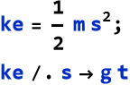
This shows kinetic energy with a gravity-driven speed—perfect for a falling object.

Need to swap more than one thing? Use a list of rules. Imagine a position function,

(5.9)

ans we want to make these specific substitutions,

(5.10)

We write

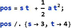
This might be a projectile’s position, with 12 meters from the initial motion and 8a from acceleration.

Substitutions get fancier with patterns. Say you’re working with a the expression,

(5.11)

and you want to replace with a new term, r. We write:

Order Matters: Substitutions apply left to right in a list—later rules override earlier ones if variables overlap. No Simplification: /. just replaces; use Simplify[] after if needed (e.g., x^2 + 2 /. x^2 -> 4 won’t add to 6 without Simplify[]). Flexibility: Rules can be stored, like rule = {v -> a t}, then reused with expr /. rule. Substitutions with /. are your shapeshifting tool—adapting expressions to fit your needs.

Problem 5.26: A speed expression is given as . What is the speed after 3 seconds? Play around with different accelerations and different initial speeds.

Energy Conservation

We have already seen many cases of kinetic energy. There is another kind of energy that an object has just by being where it is. We can call this the potential energy of an object. For example, the potential energy of an object being pulled down by gravity can be calculated by writing the mass of the object, the acceleration due to gravity, and the height of the object above ground level, h,

(5.12)

There is also potential energy contained in a compressed or extended spring, where we write the length of compression as x and extension as -x,

(5.13)

It turns out that the total of the energies present in a system is a number that never changes. For simple systems we have kinetic energy and potential energy. The total energy can be symbolized by E,

(5.14)

We have codified the principle that the total energy is a constant in what we call the conservation of energy law. If we measure the total energy before we do something, it will be the same as after we do it. Note that the kinetic energy and the potential energy might change individually, but the total remains the same.

If we have an object subject to gravity, then the total energy will be

(5.15)

We can substitute in the proper values for these energies. Recall from (4.16) and (5.8) that the kinetic energy is,

(5.16)

If we adopt (5.12) for the potential energy, this will give us the total energy

(5.17)

There is an important convention to use here. We have stated that the acceleration due to gravity is approximately -10 of acceleration, We can also say that the acceleration is simply 10 and place the minus sign on the g symbol, where we get,

(5.18)

We could factor the masses to get,

(5.19)

If we turn to MMA we can see if it can handle this.

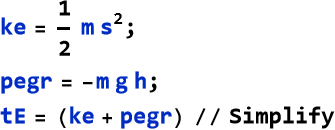
Note that MMA even factored out the 1/2, in so doing it then multiplied the potential energy term by 2.  We rewrite (5.19),

(5.20)

We have played around with expressions for speed and for the position of a falling object. We can adapt (5.7) by replacing a with -g,

(5.21)

We can write the position of a falling body,

(5.22)

If we simply drop the object, then , or,

(5.23)

What happens when we substitute these values into (5.20)?

That’s pretty complicated. Let’s try expanding this.

We can apply the command TraditionalForm.

If we look at this long enough we will see that it is just our original expression T + U. So we can apply this to (5.20)

(5.24)

This an example of deriving an expression for a physical situation.

Terms and Definitions

Term/Definition 5.39 Potential energy (symbol U): Energy an object possesses due to its position or configuration.

Term/Definition 5.40 Gravitational potential energy ): Potential energy due to gravity; calculated as m g h (or -m g h depending on sign convention).

Term/Definition 5.41 Spring potential energy ): Potential energy stored in a compressed or extended spring; calculated as .

Term/Definition 5.42 Total energy (E): The sum of kinetic and potential energies in a system (E = T + U).

Assumptions (the implicit beliefs the author relies on)

Assumption 5.19: Systems can be simple (only kinetic + potential energy, no friction/losses).

Assumption 5.20: Total energy is conserved in such systems (kinetic and potential interchange but sum constant).

Principles

Principle 5.4: Energy exists in different forms; we have identified kinetic (motion) and potential (position/configuration).

Principle 5.5: Conservation of energy is a fundamental law—total energy before something happens = total energy after something happens.

Exercise 5.26: Begin with Term/Definition 5.39 and copy it into your notebook. Reflect on its meaning for a few minutes. Note any thoughts that come to mind. How would you explain this to someone sitting in front of you. Write this down. Then do this for each term/definition, assumption, and principle.

Rest Energy

Rest energy is one of the most mind-blowing ideas in physics, courtesy of Albert Einstein’s special theory of relativity. It says that even when an object sits still, it has energy locked in its mass—expressed as a relationship between mass m and the speed of light in a vacuum c, this value is approximately 3 × . Recall that we can write the word approximately as  a curly equals sign (or [ESC] the double tilde then [ESC] in MMA), thus we write . The expression for this rest energy is

(5.25)

This rest energy is the baseline for all energy in relativity, and WL lets you explore it, tweak it, and connect it to other forms using tools like substitutions, Expand[], Factor[], Collect[], and FullSimplify. Let’s dive in and see how this famous equation plays out computationally.

Start with the iconic formula.

For a unit of mass this results in a whopping 9 × , assuming we have some way to get at it.

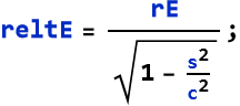
In relativity, total energy includes rest energy plus kinetic energy for a moving object. The full expression is:

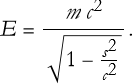
(5.26)

This is the rest energy divided by the square root of the quantity 1 less the fraction of the speed of the object squared to the speed of light squared.

For an object at rest, we get this result:

Not surprisingly, this is just the rest energy. As s increases, the denominator shrinks, boosting total energy above the rest value.

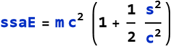
For small speeds (much less than c), the total energy approximates to,

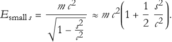
(5.27)

We can use WL to find out what this is really saying

Let’s see what happens if we expand this.

We see that this is just the sum of the rest energy and kinetic energy.

Terms and Definitions

Term/Definition 5.43 Rest energy ): The energy inherent in an object’s mass when at rest; given by .

Term/Definition 5.44 Speed of light (symbol c): The constant speed of light in vacuum; approximately 3 × m/s (denoted c ≈ 3 × m ).

Term/Definition 5.45 Total energy (symbol E): In special relativity, the energy of a moving object; .

Assumptions (the implicit beliefs the author relies on)

Assumption 5.21: For speeds << c, relativistic effects approximate classical kinetic energy ().

Principles

Principle 5.6: Rest energy is inherent in mass.

Principle 5.7: As speed increases toward c, total energy grows without bound (denominator → 0).

Exercise 5.27: Begin with Term/Definition 5.34 and copy it into your notebook. Reflect on its meaning for a few minutes. Note any thoughts that come to mind. How would you explain this to someone sitting in front of you. Write this down. Then do this for each term/definition, assumption, and principle.

Wolfram Documentation

The Wolfram Language is a vast toolbox, and we’ve only scratched the surface. But what happens when you need more details, examples, or new tricks? That’s where the Wolfram Documentation comes in—a treasure trove of information built right into the Wolfram Language. It’s your guidebook for mastering the language, packed with explanations and examples. Let’s explore how to use it and why it’s a must for your journey.

The Wolfram Documentation is a built-in resource detailing every command, function, and feature of the Wolfram Language. Think of it as a manual combined with an encyclopedia—searchable, interactive, and constantly updated. It covers syntax, options, and real-world uses, often with examples you can tweak. For physics amateurs, it’s a lifeline to bridge math and computation.

In Mathematica: Type a command, press F1 (or Ctrl+Shift+D on some systems), and a help window pops up. Try it out for yourself. You can also right click on the command and then click on Get Help. On the web you can visit the page https://reference.wolfram.com/language/ where you can browse through different features (this is especially helpful if you are using the free Wolfram Engine). You can access the same system within MMA by going to the Help Tab, then clicking Wolfram Documentation.

You can also start a command with ? For example

Problem 5.28: Look up the commands we have used throughout this lesson and see if you understand them.

Problem 5.29: Read through the workflows for Working in Notebooks and Using the Wolfram Language.

Summary

Write a summary of this lesson as an exercise.

For Further Study

Bruce F. Torrence, Eve A. Torrence, (2019), The Student’s Introduction to Mathematica and the Wolfram Language, Cambridge University Press, 3rd Edition.