Lesson 24 Calculus 5: Applications and Techniques of Integration

“What one fool can do, another can.”— Silvanus P. Thompson

“God does not care about our mathematical difficulties. He integrates empirically.”— Albert Einstein

Introduction

You have now crossed the fundamental threshold. In the previous you learned the integral as the precise mathematical expression of accumulated change, and you applied it immediately to the work done by a variable force. That was the payoff—the moment when the abstract symbol ∫ became a physical tool. This Lesson is where integration truly comes alive in theoretical physics. Here we move beyond the basic machinery and explore its astonishing range of applications and the more powerful techniques needed when the problems become realistic. You will calculate areas between curves, volumes and surface areas of solids of revolution, centers of mass of continuous objects, hydrostatic forces on dams and submarines, and the first gentle steps into differential equations—the true heart of mathematical physics. You will master advanced integration methods—trigonometric substitution, partial fractions, hyperbolic functions, and rationalizing substitutions—that let you attack integrals.

We will also confront the realities of the real world; improper integrals over infinite domains, singularities, discontinuities, and questions of convergence. These ideas are not mere technicalities. They appear directly in radioactive decay, probability densities near the origin, wave diffraction (the famous Dirichlet integral), and the normalization of probability distributions over infinite space.

By the end of this lesson you will have a versatile integration toolkit and—more importantly—a deepened physical intuition about how nature sums infinitesimal contributions to produce observable reality. The techniques you learn here will return again and again as you advance into theoretical physics.

We begin with geometric applications (area, volume, surface area) that build confidence and visualization skill, then move to classic physics problems (center of mass, hydrostatic pressure), before turning to the more sophisticated techniques and the subtle behavior of integrals at infinity and at singularities. Along the way we will pause to see how these same ideas govern radioactive half-life, probability, and numerical methods when analytic solutions become impossible.

The integral is no longer just a calculator. It is becoming one of your most reliable lenses for seeing the universe.

Let us begin.

Area Between Curves

You have already learned that the definite integral gives the net signed area under a single curve. Nature, however, rarely presents us with only one curve. The work done by a spring against gravity, the region between a planetary orbit and its circular approximation—all involve the difference between two functions.

The area between curves is the natural extension of the single-curve integral. It shows how integration measures accumulated difference, and it provides beautiful, concrete practice before we move on to volumes, centers of mass, and the more advanced techniques later in this lesson. Mastery here builds both geometric intuition and confidence in setting up integrals from physical descriptions.

Definition 24.1 Area Between Curves: Let f(x) and g(x) be continuous functions on the closed interval [a, b] with f(x)≥g(x) for all x in [a, b]. The area A of the region between the two curves is given by

(24.1)

If the curves cross within the interval, split the integral at the intersection points so that the upper function is always on top in each subinterval.

In the (rare) case where the region is described with respect to y, we integrate with respect to y

(24.2)

The integrand f(x)−g(x) is the vertical distance between the upper and lower curves at each x. Multiplying by the infinitesimal width dx gives a thin rectangular strip. The integral sums these strips to produce the exact total area. The sign is automatic: positive when f>g, negative when the curves reverse (which is why we usually split at crossings).

Suppose the force from a nonlinear spring is and a linear restoring force is . The “extra” work stored due to the cubic term between x=0 and is exactly the area between the two curves

(24.3)

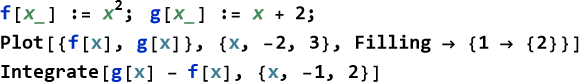
As another example, say we need to find the area between and y=x+2 from their leftmost to rightmost intersection. First solve with x=-1 and x=2. So on [-1,2] y=x+2 is above . Thus

(24.4)

Algorithm 24.1 General Procedure for Determining the Area Between Curves:

Sketch the curves and find all intersection points.

Determine which function is upper and which is lower in each subinterval.

Set up the integral(s) using Definition 24.1.

Evaluate and interpret the result physically when possible (work, charge, probability mass, etc.).

We can see this in the Wolfram Language.

Definitions

Definition 24.2 Net Signed Area: The integral without absolute value; positive and negative contributions can cancel.

Definition 24.3 Intersection Points: Solutions to f(x)=g(x), used to split integrals when curves cross.

Axioms

Axiom 24.1: Infinitesimal rectangular strips of height ∣f(x)−g(x)∣ and width dx approximate the true area, with the error vanishing as dx→0.

Principles  

Principle 24.1: The area between two curves is the accumulated difference of the two functions. Integration automatically performs this accumulation.

Principle 24.2: Try to sketch first. Visual identification of upper and lower functions prevents sign errors.

Principle 24.3: Physical quantities (work difference, charge between potentials, probability between distributions) are often computed as areas between relevant curves.

Theorems  

Theorem 24.1 Area Additivity: If [a,b] is split at c, then

(24.5)

Proof of Theorem 24.1: This is a direct proof. Let F(x) be any antiderivative of f(x)−g(x). By the Fundamental Theorem of Calculus,

(24.6)

and

(24.7)

and

(24.8)

Adding the last two equations gives

(24.9)

The F(c) terms cancel. QED

Exercise 24.1: Begin with Definition 24.1. Copy this into your notebook. Reflect on its meaning for a few minutes. Note any thoughts that come to mind. How would you explain this to someone sitting in front of you. Write this down. Do this for the algorithm, each definition, each principle, the theorem, and the proof.

Exercise 24.2: Sketch and compute the area between y=sin⁡ x  and y=cos x from x=0 to x=π/4. Interpret the result.

Exercise 24.3: Find the total area between and the x-axis from x=−2 to x=2 (note the curve crosses the axis).

Exercise 24.4: A particle moves under two different force laws and . Compute the difference in work done from x=0 to x=3 as the area between the curves.

Arc Length

You already know how to compute straight-line distances. But many important curves in physics—the shape of a hanging chain, the trajectory of a projectile, the path of a light ray, and so on—are not straight. So, we can see that it is important to know how to measure the actual length along a curving path.

The idea is simple and beautiful. Imagine breaking the curve into many very small pieces. Each piece is so short that it looks almost like a straight line. You can find the length of each tiny straight piece using the Pythagorean theorem, then add them all up. In the limit as the pieces become infinitesimally small, this sum becomes a definite integral.

Suppose we have a smooth curve given by y=f(x) from x=a to x=b. Divide the interval into small widths Δ x. Over each small interval the curve rises by a small amount Δ y. The little piece of curve then forms the hypotenuse of a tiny right triangle with legs Δ x and Δ y. Its length is therefore

(24.10)

Using the Mean Value Theorem, Δy=f'(c) for some c between the endpoints of the small interval. Substituting and simplifying gives a factor of multiplied by Δ x.

Summing all these tiny lengths and taking the limit as the pieces shrink to zero produces the exact length of the curve.

Theorem 24.2 Arc Length: Let f(x) be continuously differentiable on [a, b]. The length L of the curve y=f(x) from x=a to x=b is

(24.11)

If the curve is given as x=g(y), the formula becomes

(24.12)

The quantity tells you how much longer the actual path is compared to the horizontal distance dx. When the curve is nearly flat the factor is almost 1. When the curve is steep the factor grows, correctly making the path longer. This is exactly the stretching factor you need when a curve is later rotated to form a surface.

Proof of Theorem 24.2: This is a direct proof. The infinitesimal length element along the curve is

(24.13)

Integrating this element from x=a to x=b gives the total arc length directly. QED

Let’s say we want to determine the length of a straight line y=m x+c

(24.14)

Exercise 24.5: Show that this result becomes the familiar distance formula.

Let’s say we want to find the length of a quarter circle. Here from x=0 to x=r, the integral evaluates to π r/2, exactly one-quarter of the circumference.

Algorithm 24.2 General Procedure for Arc Length:

Express the curve in the form y=f(x) or x=g(y).

Compute the derivative.

Form the integrand (or the corresponding form in y).  

Integrate.

We can see this sort of thing in Wolfram Language.

Definitions

Definition 24.4 Arc Length: The actual distance measured along a curve between two points.

Definition 24.5 Rectifiable Curve: A curve whose length can be found by this limiting process (the integral exists and is finite).

Axioms

Axiom 24.2: Length is additive: the whole curve’s length equals the sum of the lengths of its pieces.

Axiom 24.3: The shortest path between any two points is the straight line connecting them.

Principle

Principle 24.4: The infinitesimal length element along a curve is .

Theorems

Theorem 24.3 The arc length is independent of how we parametrize the curve.

Exercise 24.6: Begin with Theorem 24.2. Copy this into your notebook. Reflect on its meaning for a few minutes. Note any thoughts that come to mind. How would you explain this to someone sitting in front of you. Write this down. Do this for each definition, axiom, principle, algorithm, theorem, and proof.

Exercise 24.7: Compute the arc length of from x=0 to x=4.

Exercise 24.8: Verify that the formula gives the correct length for any straight line.

Exercise 24.9 Set up the integral for the length of y=sin x from x=0 to x=π.

Exercise 24.10 Find the arc length of the catenary y=cosh⁡ x  from x=−1 to x=1.

Exercise 24.11 Describe a real physical curve (a road, a cable, a particle path) and write the arc-length integral for it.

Surfaces and Volumes of Revolution

You have just learned how to compute areas between curves by integrating vertical or horizontal differences. Now we rotate those curves around an axis. A single line segment rotated about an axis generates a disk, a washer, or a cylindrical shell. A curve rotated about an axis sweeps out an entire solid of revolution or a surface of revolution. These solids appear often in physics; flywheels, pistons, spherical tanks, lenses, and even stars modeled as rotating fluids We now give you three powerful methods for finding volumes—disk, washer, and shell—plus the formula for surface area. Each method is simply integration applied to a different way of slicing the solid into infinitesimal pieces. Mastery here will pay immediate dividends when you reach center of mass, hydrostatics, and later when you work in cylindrical or spherical coordinates.

The Disk Method for calculating Volume: When a region bounded by the curve y=f(x), the x-axis, and the lines x=a and x=b  is rotated about the x-axis, each cross-section perpendicular to the x-axis is a disk of radius f(x).

Theorem 24.4 Volume by Disks (about x-axis):

(24.15)

Proof of Theorem 24.4: This is a direct proof. Let A(x) be the cross-sectional area of the solid at position x. For the disk method, every cross-section perpendicular to the x-axis is a disk of radius f(x), so

(24.16)

The volume of the entire solid is the integral of the cross-sectional area from a to b, resulting in (24.15). QED

Each thin disk represents an infinitesimal “slice” of the solid. The factor is the area of the circular face, and multiplying by dx (the thickness) gives its volume. Integration simply adds up all these infinitesimal volumes. Nature performs this summation automatically when a real object (a turned wooden bowl, a star, a flywheel rim) is formed by rotation. The integral merely computes what nature has already done.

Here is a demonstration of this method. Note the use of the command RevolutionPlot3D;function, range,options].

Here is a more general demonstration allowing you to choose one of several functions.

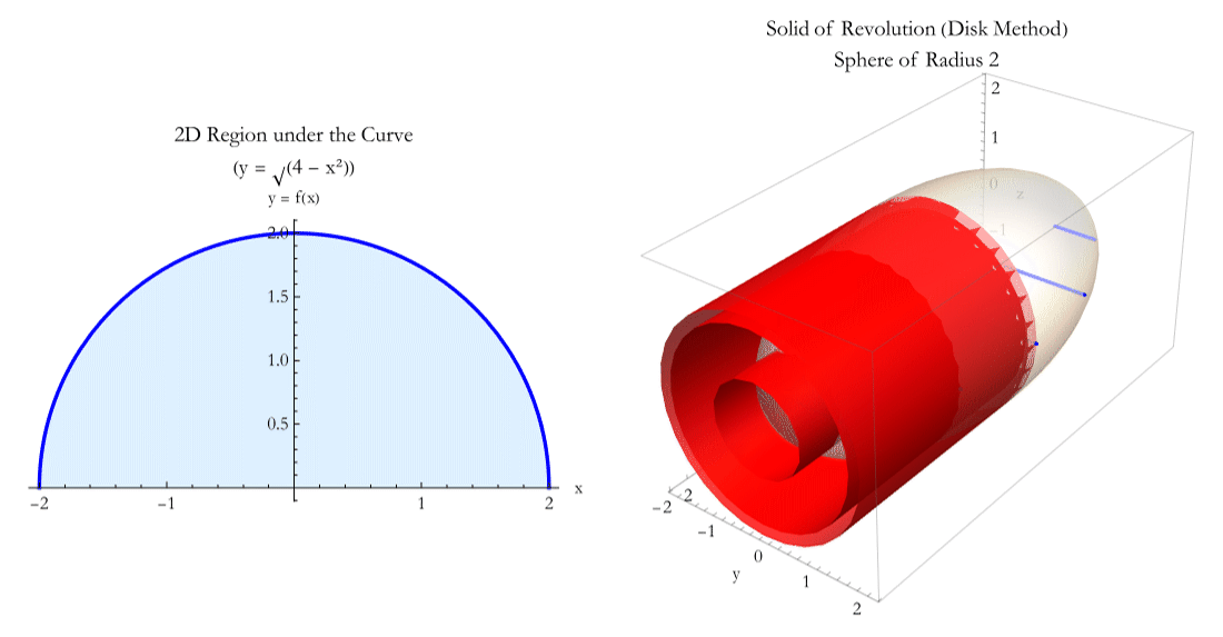
The Washer Method of Calculating Volume: When the region is between two curves y=f(x) (outer) and y=g(x) (inner) rotated about the x-axis, each slice is a washer (disk with a hole—an annulus).

Theorem 24.5 Volume by Washers (about x-axis):

(24.17)

(The same logic applies when rotating about the y-axis; simply integrate with respect to y and use x as the radius function.)

Each thin washer is a slice of material with a hole in the middle. The integral automatically subtracts the empty inner volume at every point. This is exactly what happens when you bore a hole through a cylinder, cast a pipe, or form a toroidal tank—nature removes the inner material, and the integral computes the remaining volume by subtracting the areas before multiplying by thickness.

Exercise 24.12: Prove Theorem 24.5 using Theorem 24.4.

Here is an example allowing you to choose from several functions.

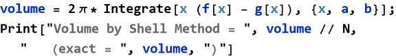
Shell Method: Instead of slicing perpendicular to the axis of rotation, we use thin cylindrical shells parallel to the axis. This is often easier when rotating about the y-axis or when the function is given as x in terms of y.

Theorem 24.6 Volume by Shells (about y-axis): For a region between x=f(y) and x=g(y) from y = c to y = d,

(24.18)

(When rotating about the x-axis the radius becomes x and we integrate with respect to x.)

Proof of Theorem 24.6: This is a direct proof. Imagine a solid built from concentric thin cylindrical shells centered on the y-axis. At radius x, the shell has

(24.19)

Then it has,

(24.20)

With

(24.21)

Its infinitesimal volume is therefore

(24.22)

Integrating these infinitesimal shell volumes from x=a to x=b gives the total volume. This result is (24.18). QED

Each thin shell is like a layer of material wrapped around the axis of rotation. The factor 2π x is the circumference at radius x, the term [f(x)−g(x)] is the height of the strip being rotated, and dx is its thickness. The integral simply adds up the volumes of all these concentric layers.This method is often easier when the region is described as a function of x and we are rotating about the y-axis, because we avoid having to solve for inverse functions.

When g(x)=0, the shell formula reduces to , the volume generated by rotating the area under a single curve about the y-axis.

The shell method is fully equivalent to the disk/washer method—they must always give the same numerical result when both can be applied—but one may be far simpler to compute than the other depending on the geometry.

Principle 24.5: Choose the method that produces the simplest integrand and easiest limits. Sketching the solid and a typical slice is essential.

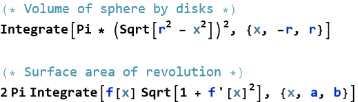
Surface Area of Revolution When a curve y=f(x) from x=a to x=b is rotated about the x-axis, the surface area generated is

Theorem 24.7 Surface Area of Revolution (about x-axis):

(24.23)

Proof of Theorem 24.7: This is a direct proof. Divide the interval [a, b] into n subintervals, each of width . Let be a sample point in the ith subinterval.

At this small segment the curve goes from height to .

The vertical change is .

The horizontal change is .

When this small piece of curve is rotated about the x-axis, it generates a surface that closely approximates the lateral surface of a frustum (truncated cone) with the and the , and the slant height = the straight-line distance between the two points on the curve. The lateral surface area of a frustum of a cone is

(24.24)

where is the slant height of the frustum.

(24.25)

By the Mean Value Theorem (since f is differentiable), there exists some in  in such that

(24.26)

Thus

(24.27)

The approximate surface area element becomes

(24.28)

For small , (by continuity of f). Therefore

(24.29)

Summing over all subintervals gives the total approximate surface area

(24.30)

This is a Riemann sum. As n→∞ and , both and approach the same point in the limit, and the sum converges to the definite integral (24.18).QED

Each tiny piece of the curve, when rotated, sweeps out a narrow band on the surface. We approximate that band as the side of a frustum of a cone. The factor 2π f(x) is essentially the average circumference at that location, and the term accounts for the true slanted length of the curve element (not just the horizontal dx). The integral sums all these infinitesimal bands.

When the curve is very flat (f'(x)≈0), the formula reduces to the lateral area of a cylinder: S≈2π r(b−a), as expected.

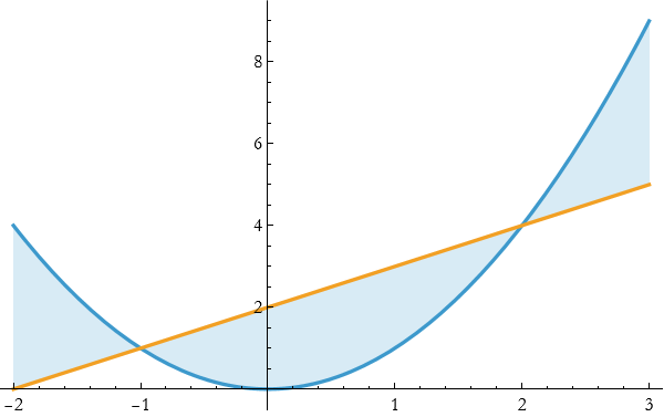
Let’s say we want to create a sphere by rotating a semicircle. Rotate the upper half of the circle about the x-axis from −r to r. Using disks

(24.31)

(the familiar volume of a sphere). Using the surface-area formula on the same semicircle yields .

Algorithm 24.2 General Procedure for Volumes:

Sketch the region and the axis of rotation.

Decide: disk/washer (slice perpendicular to axis) or shell (slice parallel to axis).

Determine the radius and height (or thickness) of each slice.

Write the volume element and integrate.

For surface area, use the arc-length element times circumference.

We can see an example of this in the Wolfram Language.

Definitions

Definition 24.6 Solid of Revolution: A three-dimensional object generated by rotating a two-dimensional region about an axis.

Definition 24.7 Disk / Washer: Cross-sectional slice perpendicular to the axis of rotation.

Definition 24.8 Cylindrical Shell: Thin cylindrical layer parallel to the axis of rotation.

Definition 24.9 Surface of Revolution: The surface traced by a curve rotated about an axis.

Axioms

Axiom 24.4: Volume is additive over non-overlapping slices.

Axiom 24.5: The volume of a thin slice (disk, washer, or shell) approximates the true volume, with error vanishing as thickness → 0.

Principles

Principle 24.6: The squared radius in the disk/washer method comes from the area of a circle; the 2π r in the shell method comes from the circumference.

Principle 24.7: Surface area integrals combine the circumference at each point with the infinitesimal arc length along the generating curve.

Theorems

Theorem 24.8: The disk, washer, and shell methods are all equivalent; they yield identical results when applied correctly to the same solid.

Exercise 24.13: Prove Theorem 24.8.

Exercise 24.14: Begin with Theorem 24.4. Copy this into your notebook. Reflect on its meaning for a few minutes. Note any thoughts that come to mind. How would you explain this to someone sitting in front of you. Write this down. Do this for each definition, axiom, principle, algorithm, theorem, and proof.

Exercise 24.15: Use the disk method to derive the volume of a right circular cone of radius R and height H.

Exercise 24.16: Use the shell method to find the volume generated by rotating from x = 0 to x = 4 about the y-axis.

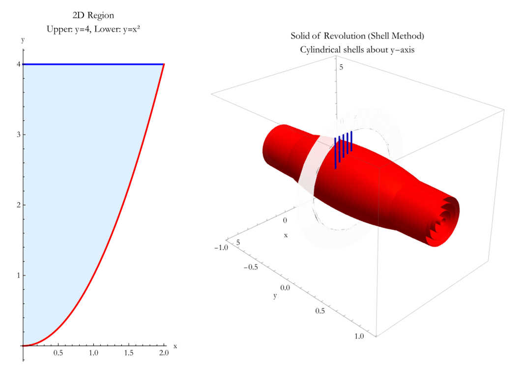
Exercise 24.17: A region bounded by , y = 4, and x = 0 is rotated about the y-axis. Compute the volume using both washer and shell methods and verify they agree.

Exercise 24.18: Find the surface area generated by rotating from x = 0 to x = 1 about the x-axis. (This will require a substitution.)

Exercise 24.19: Think of a real physical object (flywheel rim, spherical pressure vessel, paraboloidal mirror). Describe the generating curve, choose a method, and set up the integral for its volume or surface area.These methods are not isolated tricks — they are fundamental ways of summing infinitesimal contributions in three dimensions. You will meet them again when computing moments of inertia, centers of mass, and potentials in later lessons.

Mass Distributions and Center of Mass

You have now learned to sum infinitesimal contributions to find areas between curves, arc lengths, volumes, and surface areas of solids of revolution. We now turn to one of the most physically powerful applications of integration, the study of how mass is distributed in real objects.

Real bodies are rarely uniform blocks. Mass is spread along a wire, across a plate, or throughout a volume—sometimes evenly, often not. The the single point that behaves as if the entire mass of the object were located there when the object moves as a whole is what we call the center of mass. It is the balance point of the object and the natural reference for describing straight-line motion.

To reach this idea we first need two closely related concepts. The first is a way of adding up a quantity when not every part is equally important—what we call a weighted measure. We multiply each small piece by a weight that reflects its significance (often its distance from a chosen reference) before summing.

Think of it this way, a small mass far from an axis has a much greater effect on balance or rotation than the same mass close to the axis. The farther piece receives a larger weight in the sum. Integration performs this weighting and accumulation automatically for continuous distributions.

Definition 24.10 Moment: The moment of a distributed quantity about a reference point or axis is the weighted sum obtained by multiplying each infinitesimal element by its distance from that reference.

For a quantity distributed along a line with density λ(x), the first moment about x=0
is

(24.32)

For a region between curves y=f(x) and y=g(x) with area density σ(x), the moments about the coordinate axes are expressed using the single integrals you already know.

The first moment tells us “how much quantity is present and how far, on average, it lies from the reference.”

Definition 24.11 The Center of Mass: The center of mass of an object is the point where the total first moment of mass is exactly accounted for by placing the entire mass at that single location.

Say we have a thin rod or wire. We can think of it as one-dimensional. With linear density λ(x) from x=a to x=b. So, the total mass is

(24.33)

Then the center of mass is located at

(24.34)

For the region between y=f(x) and y=g(x), where (f(x)≥g(x)) from x=a to x=b with areal density σ(x). The total mass is,

(24.35)

The center of mass coordinates are then,

(24.36)

and

(24.37)

When the density is constant (λ or σ is the same everywhere), the center of mass coincides with the geometric center of the shape, called the centroid. In this case the formulas simplify by replacing with the total area A and removing σ from the integrals.

There is a set of beautiful results that connect the center of mass (or centroid) directly to the volumes and surfaces you calculated earlier.

Theorem 24.9 Pappus’s Centroid Theorem for Volume: A plane region of area A (or mass ) whose center of mass (or centroid) lies at distance from an external axis generates a solid of volume

(24.38)

when rotated about that axis.

Proof of Theorem 24.9: This is a direct proof. We prove it using the shell method and the definition of the centroid. For simplicity, assume the region R lies in the x y-plane to the right of the y-axis and is rotated about the y-axis. (The argument is identical for any external axis.)

Let the region be bounded by x=f(y) (right curve) and x=g(y) (left curve, possibly 0), from y=c to y=d, with f(y)≥g(y)≥0.

The area of R is

(24.39)

The x-coordinate of the centroid (distance from the axis of rotation) is

(24.40)

where is the centroid of each thin horizontal strip.

Now rotate R about the y-axis and compute the volume using the shell method. Consider a thin horizontal strip at height y, of width dy, and length f(y)−g(y). When rotated about the y-axis, this strip sweeps out a thin cylindrical shell of

(24.41)

(24.42)

and

(24.43)

The volume of this thin shell is

(24.44)

Integrating over the whole region gives the total volume

(24.45)

Compare this with the definition of the centroid distance

(24.46)

Therefore

(24.47)

Substituting back yields

(24.48)

Since is exactly the distance from the centroid to the axis of rotation in the general statement), we have

(24.49)

QED

Theorem 24.10 Pappus’s Centroid Theorem for Surface Area: A plane curve of length L whose centroid lies at distance from an external axis generates a surface of area

(24.50)

when rotated about that axis.

Exercise 24.20: Prove Theorem 24.10.

Principles

Principle 24.9: A moment is a weighted measure, each infinitesimal element is multiplied by its distance from the reference before integration.

Principle 24.10: The center of mass is the weighted average position of the mass.

Principle 24.11: For uniform density the center of mass and centroid are identical.

Principle 24.12: Once you know the distance from the center of mass (or centroid) to an axis, Pappus’s theorems turn complicated revolution problems into simple multiplication.

Exercise 24.21: Begin with Definition 24.10. Copy this into your notebook. Reflect on its meaning for a few minutes. Note any thoughts that come to mind. How would you explain this to someone sitting in front of you. Write this down. Do this for each definition, principle, theorem, and proof.

Exercise 24.22: A thin rod of length L lies along the x-axis from x=0 to x=L with linear density , where is a positive constant.  
    1) Find the total mass.
    2) Find the center of mass.
    3) Interpret the result: does the center of mass lie to the left or right of the midpoint? Why?

Exercise 24.23: Find the centroid of the triangular region bounded by y=0, y=h(1−x/b), and x=b (a right triangle with base b and height h). Verify that the result matches the known geometric rule that the centroid lies at one-third the height from the base.

Exercise 24.24: The region between and y=x from x=0 to x=1 has uniform density. Find its centroid .

Exercise 24.25: A thin plate has variable area density in the region between y=0 and y=sin x from x=0 to x=π.
    1) Set up the integrals for the total mass and the center of mass coordinates and .
    2) Do not evaluate the integrals. Explain qualitatively where you expect and to lie and why.

Exercise 24.26: The region between y=x and from x=0 to x=1 has area A=1/6. Its centroid distance from the y-axis is .  
Use Pappus’s Volume Theorem to find the volume of the solid generated when this region is rotated about the y-axis. Compare your result with the volume you would obtain using the shell method (optional challenge).

Exercise 24.27: Consider a hammer. The head is much denser and heavier than the wooden handle.
    1) Qualitatively sketch where you expect the center of mass to be located and explain why.
    2) How does this affect the way a carpenter swings the hammer?
    3)  If you wanted to make the hammer easier to swing for long periods, where would you add a small counterweight, and why? Use the ideas of moment and center of mass in your             reasoning.

Hydrostatic Pressure

You have learned to find centers of mass and centroids by summing weighted infinitesimal contributions. Now we apply the same idea to fluids at rest. In a stationary fluid, pressure increases steadily with depth. This seemingly simple fact has powerful consequences, it explains why dams are thicker at the bottom, why submarines have depth limits, and how forces on submerged surfaces can be calculated exactly using integration.

You will derive the fundamental relation between pressure and depth, learn how to compute the total force on any submerged surface, and see how the center of pressure (the point where the total force effectively acts) is found using moments.

Definition 24.12 Pressure: Pressure P at a point in a fluid is the force per unit area acting perpendicular to any surface passing through that point

(24.51)

Definition 24.13 Hydrostatic Pressure: In a fluid at rest (hydrostatic equilibrium), the pressure at a depth h below the free surface is

(24.52)

where is the pressure at the surface (usually atmospheric pressure), ρ is the fluid density (assumed constant for incompressible liquids), g is the acceleration due to gravity, and h is the vertical depth.

The term ρ g h is called gauge pressure.

When pressure varies with depth, the total force on a submerged plate or dam is no longer simply pressure times area. We must integrate.

Theorem 24.11 Force on a Submerged Surface: The total force F on a submerged surface is the integral of the pressure over the area (note that this integral is denoted and is the first moment of the area with respect to the free surface)

(24.53)

If atmospheric pressure acts on both sides (or we use gauge pressure), it often cancels, leaving

(24.54)

Proof of Theorem 24.11: This is a direct proof. Consider an arbitrary submerged surface S. Divide the surface into many tiny area elements dA, each small enough that the pressure over it can be considered nearly constant.

At the location of the ith element, the vertical depth below the free surface is . By the hydrostatic pressure relation in an incompressible fluid at rest,

(24.55)

where is the pressure at the free surface (usually atmospheric pressure), ρ is the constant fluid density, and g is the acceleration due to gravity.

The infinitesimal force on this small element is pressure times area

(24.56)

The total force on the entire surface is the sum of all these small forces

(24.57)

The first sum is simply the total area A of the surface. Taking the limit as the number of elements goes to infinity and each , the sums become definite integrals

(24.58)

This is the exact expression for the total force.

When atmospheric pressure acts on both sides of the surface (as is typical for dams, gates, and submarine windows), it cancels out. In that case we work with gauge pressure , and the total force simplifies to

(24.59)

Where is the first moment of the area of the submerged surface with respect to the free surface of the fluid. QED

The center of pressure is the point on the surface where the total force appears to act. It is found using the second moment (also called the moment of inertia) of the area.

For a vertical surface, the depth of the center of pressure is

(24.60)

where is the depth of the centroid and is the second moment of area about the horizontal axis through the centroid.

Algorithm 24.4 General Procedure for Pressure

Sketch the surface and choose a coordinate system (often depth h).

Express the pressure as a function of position on the surface.

Set up the integral F=∫P dA (use horizontal strips for vertical surfaces).

For center of pressure, compute the moment of the force and divide by total force.

For example a rectangular dam of width w and height H holds water to its full height. Using gauge pressure, the total force is

(24.61)

The center of pressure lies at 2/3H below the surface (deeper than the centroid at H/2).

Definitions

Definition 24.14 Gauge Pressure: Pressure above atmospheric pressure (ρ g h).

Definition 24.15 Center of Pressure: The point where the total hydrostatic force effectively acts.

Definition 24.16 Free Surface: The free surface of a liquid is the interface between the liquid and the air (or other gas) above it, where the pressure is equal to the atmospheric pressure .

At a free surface:

The pressure is (usually taken as 1 atm or 101325 Pa).

The surface is “free” to move and adjust its shape under gravity and external forces.

In hydrostatic equilibrium, the free surface is horizontal (perpendicular to gravity) unless the container is accelerating.

Axioms

Axiom 24.6: A fluid at rest experiences only normal forces.

Axiom 24.7 Pascal’s Principle: Pressure at a point in a static fluid is the same in all directions.

Principles

Principle 24.13: In a static fluid, pressure increases linearly with depth.

Principle 24.14: The total force on a surface is the integral of pressure over area—thus pressure is not uniform.

Principle 24.15: The center of pressure is always deeper than the centroid for vertical surfaces because pressure increases downward.

Principle 24.16: Atmospheric pressure often cancels when it acts on both sides of a surface; gauge pressure simplifies calculations.

Exercise 24.28: Begin with Definition 24.12. Copy this into your notebook. Reflect on its meaning for a few minutes. Note any thoughts that come to mind. How would you explain this to someone sitting in front of you. Write this down. Do this for each definition, principle, algorithm, theorem, and proof.

Exercise 24.29: A vertical rectangular gate 2 m wide and 3 m high holds water to a depth of 2.5 m. Compute the total force on the gate (use ρ=1000 , g=9.8 ) and locate the center of pressure.

Exercise 24.30: A triangular plate with base 4 m and height 3 m is submerged vertically in water with its base at the surface. Find the total hydrostatic force and the depth of the center of pressure.

Exercise 24.31: A circular porthole of radius 0.3 m is centered 5 m below the ocean surface. Compute the total force on the porthole (use gauge pressure).

Exercise 24.32: Set up (but do not evaluate) the integral for the force on a parabolic dam whose face is given by from x=−2 to x=2 (in meters), with water to the top.

Exercise 24.33: Explain physically why the center of pressure on a vertical surface is always deeper than the centroid. What happens as the surface becomes horizontal?

Exercise 24.34: A submarine window is 8 m below the surface. If the window can safely withstand N of force, what is the maximum safe diameter for a circular window? Discuss design implications.

An Introduction to Differential Equations

You have spent many lessons learning how to use integration to sum infinitesimal contributions—work, area, volume, center of mass, hydrostatic force. These are powerful tools, but they usually give us the total result after the fact.

In the real world, many quantities change continuously over time or space according to rules that involve their own rates of change. The mathematical statement of such a rule is called a differential equation. Learning to work with differential equations is one of the most important steps in your journey toward theoretical physics. Almost every law of physics you will meet—from Newton’s second law to Schrödinger’s equation—is a differential equation.

Definition 24.17 Differential Equation: A differential equation is an equation that relates a function to one or more of its derivatives.

Definition 24.16 Order of a Differential Equation: The order is the highest derivative that appears in the equation.  First-order: involves only the first derivative.  
Second-order: involves the second derivative, and so on.

We can look at three examples.

(24.62)

the equation for exponential growth or decay.

(24.63)

the second-order equation for simple harmonic motion.

(24.64)

a generic second-order linear equation.

Definition 24.17 Solution of a Differential Equation: A function y=φ(x) is a solution if substituting it into the equation makes the equation true for all x in some interval. A general solution contains arbitrary constants (one for each order of the equation). An initial-value problem (or boundary-value problem) supplies enough extra conditions to determine those constants uniquely.

Most fundamental laws tell us how something changes:

Newton’s second law, F=m a becomes .

Radioactive decay, where the rate of change of number of atoms is proportional to the number present.

Population growth, cooling of objects, charge in a capacitor — all are differential equations.

Integration is the tool we use to solve many of them.

Algorithm 24.5 Separation of Variables (for first-order equations): If an equation can be written in the form

(24.65)

then we separate variables and integrate both sides:

(24.66)

This is one of the most useful techniques you will learn.

Algorithm 24.6 Direct Integration: For equations of the form

(24.67)

simply integrate

(24.68)

Definitions

Definition 24.18 General Solution: Solution containing all arbitrary constants.

Definition 24.19 Particular Solution: Solution satisfying specific initial or boundary conditions.

Principles

Principle 24.17:  A differential equation describes the local rule of change; its solution describes the global behavior.

Principle 24.18:  The number of arbitrary constants in the general solution equals the order of the equation.

Principle 24.19:  Initial conditions (or boundary conditions) turn a general solution into a unique particular solution that matches reality.

Principle 24.20:  Many physical laws are easier to state as differential equations than as direct relationships between quantities.

Principle 24.21:  Solving a differential equation means finding all functions that satisfy the given relation between the function and its derivatives.

Theorems

Theorem 24.12 Existence and Uniqueness–informal: For a well-behaved first-order equation y'=f(x,y) with an initial condition , there exists a unique solution in some interval around , provided f is continuous and satisfies reasonable smoothness conditions. (This is a deep result; we will use it informally for now, thus there is no proof at this time.)

Exercise 24.35: Begin with Definition 24.17. Copy this into your notebook. Reflect on its meaning for a few minutes. Note any thoughts that come to mind. How would you explain this to someone sitting in front of you. Write this down. Do this for each definition, principle, algorithm, theorem, and proof.

Exercise 24.36: Classify the following equations by order and type (linear or nonlinear):
    1) dy/dx=k y
    2)
    3)

Exercise 24.37: Solve by direct integration. Write both the general and a particular solution with y(0)=2.

Exercise 24.38: Use separation of variables to solve dy/dx=k y. Write the general solution and interpret the meaning of the constant k (positive and negative cases).

Exercise 24.39: Newton’s law of cooling says the rate of change of temperature T of an object is proportional to the difference between T and the ambient temperature
. Set up the equation and solve it using separation of variables.

Exercise 24.40: For radioactive decay we have, dN/dt=−λ N. Solve for N(t) and show that the half-life is .

Exercise 24.41: Why do you think most fundamental laws of physics are expressed as differential equations rather than direct algebraic formulas? Give at least two physical reasons.

Integration by Parts

You have already seen how the definite integral accumulates small contributions—whether for work done by a variable force, areas between curves, or hydrostatic pressure. Many important integrals in physics, however, involve the product of two different functions, position times velocity, time times exponential decay, angle times a trigonometric function, or in radioactive decay problems.

The technique called integration by parts is the integral analogue of the product rule for differentiation. It lets us transform a difficult product integral into a, usually, simpler one. Mastery of this method will unlock many integrals you will meet.

Start from the product rule for derivatives

(24.69)

Integrate both sides with respect to x. The left side becomes u v, so rearranging gives the fundamental formula.

Theorem 24.13 Integration by Parts (Indefinite Form)

(24.70)

For definite integrals the boundary terms are evaluated directly

Theorem 24.14 Integration by Parts (Definite Form)

(24.71)

Long experience with this method has resulted in practical heuristic, not a strict theorem. It is called the LIATE rule. It is a system where you can use it to classify your choice of functions u or dv in your problem. LIATE is the order of you choice of functions

L — Logarithmic functions, where differentiating gives 1/x a simper algebraic function
I — Inverse trigonometric functions, arcsin x and arccos x, differentiating gives a simpler algebraic function
A — Algebraic (polynomials), differentiating gives an algebraic function of lower power
T — Trigonometric functions, differentiating cycles through the trigonometric functions
E — Exponential functions, differentiating keeps it exponential (though this rarely simplifies the expression)

Choose u from the highest category present. Differentiate u and integrate dy. This usually makes the new integral simpler.

For example, we want to compute

(24.72)

We choose the E method. Let u=x and , and .

(24.73)

Note the integral is of opposite sign than it started out.

Let’s look at the Classic Logarithm Integral

(24.74)

We choose the L method. Let u=ln ⁡x, dv=dx. Then du=1/x dx, and , v=x.

(24.75)

Algorithm 24.7 LIATE Method:

Identify a product inside the integral.

Choose u and dy using the LIATE heuristic (be prepared to try the other way if the first choice fails).

Compute du and v.

Apply the formula (24.70)

Simplify the new integral. Repeat integration by parts if necessary.

For definite integrals, carefully evaluate the boundary term .

Definitions

Definition 24.20 Integration by Parts: The technique

(24.76)

Definition 24.21 Reduction Formula: A recursive relation obtained by integration by parts that expresses an integral in terms of a similar integral with a lower parameter.

Principles

Principle 24.22:   Integration by parts is the reverse of the product rule of differentiation.

Principle 24.23:  The goal is always to make the remaining integral simpler than the original.

Principle 24.24:  The boundary term often has direct physical meaning (final value minus initial value).

Principle 24.25: Repeated application of integration by parts can produce reduction formulas that lower the power or complexity step by step.

Principle 24.26: Choose u to be the function that becomes simpler when differentiated.  

Exercise 24.42: Begin with Definition 24.13. Copy this into your notebook. Reflect on its meaning for a few minutes. Note any thoughts that come to mind. How would you explain this to someone sitting in front of you. Write this down. Do this for each definition, principle, algorithm, theorem, and proof.

Exercise 24.43: Copy both forms of the integration by parts formula into your notebook. Next to them, write the product rule and show how one is the integral version of the other.

Exercise 24.44: Compute using integration by parts. Then evaluate the definite integral from 0 to 2.

Exercise 24.45: Find . Interpret the result geometrically as an area.

Exercise 24.46: A force varies as F(x)=x sin⁡(π x) while a particle moves from x=0 to x=1. Compute the work done using integration by parts.

Exercise 24.47: Apply integration by parts twice to . You will obtain the original integral again—solve for it algebraically (a classic trick).

Exercise 24.48: Experiment in Wolfram Language: define several products, integrate them symbolically, and plot both the integrand and the antiderivative. Try x ln⁡ x, , and x cos⁡ x.

Improper Integrals having Infinite Intervals

All the definite integrals you have worked with so far have had finite limits—from a to b. But the real world is rarely so tidy. Radioactive decay goes on forever. The probability of finding a quantum particle can stretch to infinity. Gravitational or electric potentials extend across all space. To deal with these situations we must extend the idea of the definite integral to improper integrals over infinite intervals.

This section shows you how to make sense of integrals from a to ∞, from −∞ to b, or from −∞ to ∞. You will learn when they converge (give a finite value) and when they diverge, and you will see why this matters deeply in physics.

Definition 24.21 Improper Integral over an Infinite Interval: An integral with one or both limits at infinity is called improper. We define it as a limit of ordinary definite integrals

(24.77)

provided the limit exists and is finite. If the limit exists, we say the integral converges; otherwise it diverges.

Similarly,

(24.78)

and

(24.79)

(for any convenient splitting point c).

For example, the total number of decays over infinite time is

(24.80)

This integral converges. The total “area” is finite even though time goes to infinity.

An extremely important example is that of the normal distribution over all real numbers

(24.81)

This famous integral, called the Gaussian probability, converges to 1, allowing us to normalize probabilities over infinite domains.

Algorithm 24.8 Algorithm for Evaluating Improper Integrals:

Replace the infinite limit with a finite variable (e.g., b or a).

Compute the ordinary definite integral.

Take the limit as the variable approaches infinity (or negative infinity).

If the limit is a finite number, the integral converges to that value. If the limit is ±∞ or does not exist, the integral diverges.

Definitions

Definition 24.22 Convergent Improper Integral: The limit exists and is finite.  

Definition 24.23 Divergent Improper Integral: The limit is infinite or does not exist.

Axioms

Axiom 24.8: The definite integral over a finite interval is well-defined when the function is continuous (or piecewise continuous).

Principles

Principle 24.27: An improper integral converges only if the area under the curve remains finite even when stretched to infinity.

Principle 24.28:  Rapidly decaying functions (exponentials, Gaussians, with p>1) tend to produce convergent improper integrals. Slowly decaying functions (like 1/x) often diverge.

Principle 24.29: In physics, a convergent improper integral usually means a finite total quantity (total probability = 1, total charge, total energy, etc.). Divergence often signals that our model breaks down at extreme distances or times.

Principle 24.30:  Always check convergence before trying to assign a numerical value.

Theorems

Theorem 24.15 p-test for Integrals from 1 to ∞: The integral converges if p>1 and diverges if p<=1.

Proof of Theorem 24.15: This is left for Lesson 25. We evaluate the integral as a limit

(24.82)

Case 1: p≠1

The indefinite integral is

(24.83)

Evaluating the definite integral from 1 to b

(24.84)

Now take the limit as b→∞. If p>1, then 1−p<0, so as b→∞.

Therefore

(24.85)

The limit is finite → the integral converges to 1/(p−1).

If p<1, then 1−p>0, so as b→∞.

The expression goes to ±∞ (depending on the sign of 1−p) → the integral diverges.

Case 2: p=1

(24.86)

So,

(24.87)

The integral diverges. QED

he p-test gives a simple benchmark for convergence at infinity; the integrand must decay faster than 1/x for the improper integral to converge. This is why exponential decay () always converges, while 1/x does not.

Theorem 24.15 Monotone Convergence Theorem: Let ) be a sequence of real numbers that is monotone increasing and bounded above. Then ) converges to a finite limit.

Proof of Theorem 24.15: This is a direct proof. Let be the set of all terms of the sequence.

Because the sequence is bounded above, the set S is bounded above. By the Least Upper Bound Property of the real numbers (Axiom 18.1), S has a least upper bound. Let

(24.88)

L is the smallest number that is greater than or equal to every .

We now show that . Let ε>0 be arbitrary. Since L is the least upper bound, L−ε is not an upper bound of S. Therefore there exists some index N such that

(24.89)

Because the sequence is monotone increasing, for all n≥N,

(24.90)

Also, since L is an upper bound,

(24.91)

Combining these two inequalities

(24.92)

This is exactly the definition of

(24.93)

Thus the sequence converges to its supremum L, which is finite. QED

Theorem 24.16 Comparison Test: If 0≤f(x)≤g(x) for all x≥a, then, if converges, so does . If diverges, so does .

Proof of Theorem 24.16: This is a direct proof by cases. We prove both parts using the definition of convergence of improper integrals.

Part 1: Convergence of the larger integral implies convergence of the smaller one.

Assume converges to some finite number L. That is,

(24.94)

Since 0≤f(x)≤g(x) for all x≥a, it follows that for any finite b>a,

(24.95)

The integral is a non-decreasing function of b (because f(x)≥0) and is bounded above by L.

Therefore, by the Monotone Convergence Theorem for real numbers, the limit

(24.96)

exists and is some finite number between 0 and L. Hence converges.

Part 2: Divergence of the smaller integral implies divergence of the larger one

This is the contrapositive of Part 1. Assume diverges. That means

(24.97)

Since f(x)≤g(x), we have

(24.98)

for all b>a. If the left side goes to infinity as b→∞, then the right side must also go to infinity. Therefore diverges.QED

Exercise 24.49: Begin with Definition 24.21. Copy this into your notebook. Reflect on its meaning for a few minutes. Note any thoughts that come to mind. How would you explain this to someone sitting in front of you. Write this down. Do this for each definition, axiom, principle, algorithm, theorem, and proof.

Exercise 24.50: Determine whether the following integrals converge or diverge. If convergent, evaluate them.
    1)
    2)
    3)

Exercise 24.51: Show that .

Exercise 24.52: The probability density for finding a particle in a certain state sometimes behaves as at large distances. Does the total probability converge? What does this mean physically?

Exercise 24.53: Evaluate (a famous integral connected to the arctangent function and Lorentzian distributions).

Exercise 24.54: Radioactive decay: The number of atoms remaining after time t is . Show that the total number of atoms that eventually decay is exactly by evaluating the improper integral of the decay rate from 0 to ∞.

Exercise 24.55: Why is it physically acceptable for some probability distributions to extend to infinity, yet we still require the total probability to equal 1? What would it mean if such an integral diverged?

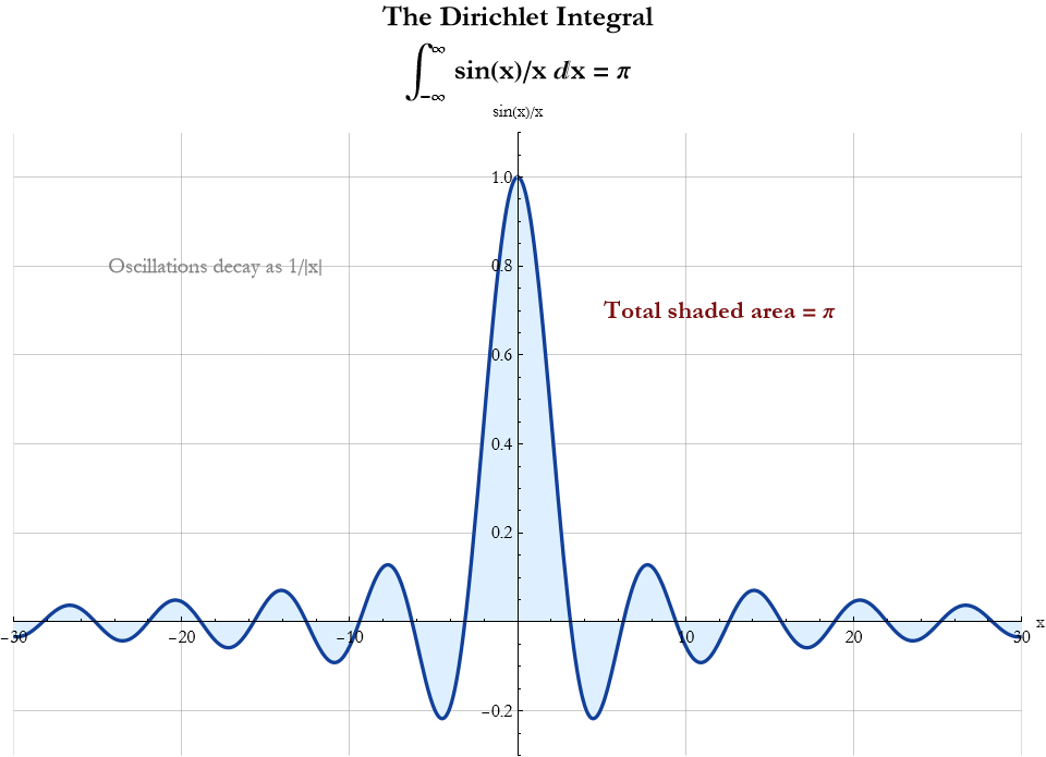
The Dirichlet Integral for Diffraction

You have now learned how to handle improper integrals over infinite intervals. Many of these integrals converge to finite values even though they stretch across all space. One of the most famous—and physically important—is the Dirichlet integral

(24.99)

This innocent-looking expression appears frequently in physics, but nowhere more beautifully than in the theory of diffraction. When light or any wave passes through a narrow slit, the diffraction pattern on a distant screen is governed by this very integral. Understanding it connects your work on improper integrals directly to one of the most striking wave phenomena in nature.

Definition 24.24 The Dirichlet Integral: The Dirichlet integral is the improper integral

(24.100)

More generally, we consider the family of integrals

(24.101)

where sgn⁡(k) is the sign of k (this gives π for k>0, −π for k<0, and 0 for k=0).The function sinc⁡(x)=sin ⁡x/x) is called the sinc function.

Consider a plane wave of wavelength λ passing through a narrow slit of width a. On a distant screen, the amplitude at an angle θ from the center is proportional to the integral of the contributions from all parts of the slit. This leads to

(24.102)

this evaluates (after some work) to a sinc function.

The intensity pattern observed on the screen is

(24.103)

where

(24.104)

The central bright fringe and the characteristic side lobes with minima at β=n π are direct consequences of the properties of the Dirichlet integral. The total “energy” spread across the entire diffraction pattern remains finite precisely because the integral converges.

Evaluating the Dirichlet integral rigorously usually requires techniques such as contour integration in the complex plane or differentiation under the integral sign (sometimes called Feynman’s trick). For now, we accept the famous result

(24.105)

as a key fact, and focus on its physical meaning and convergence (which you can now verify using the comparison test or Dirichlet test for improper integrals).

Definitions

Definition 24.25 Sinc Function: sinc⁡(x)=sin ⁡x/x.

Principles

Principle 24.31: Even though sin ⁡x/x decays slowly (only as 1/x), the rapid oscillations of sin x cause positive and negative contributions to cancel at large distances, allowing the integral to converge.

Principle 24.32: Many important physical quantities (diffraction amplitudes, Fourier transforms, probability distributions) are expressed as integrals over infinite domains. Convergence of these integrals is essential for the theory to make physical sense.

Principle 24.33: The Dirichlet integral is the bridge between the mathematics of improper integrals and the beautiful wave phenomena we observe in light, sound, and quantum mechanics.

Principle 24.34: The width of a slit and the wavelength together determine the angular spread of the diffraction pattern through the sinc function.

Exercise 24.56: Begin with Definition 24.24. Copy this into your notebook. Reflect on its meaning for a few minutes. Note any thoughts that come to mind. How would you explain this to someone sitting in front of you. Write this down. Do this for each definition and principle.

Exercise 24.57: Explain in your own words why the integral converges even though ∣sin⁡ x/x∣ behaves like 1/∣x∣ at infinity (which diverges by the p-test).

Exercise 24.58: Sketch the function sinc⁡(x) and explain qualitatively why its integral from −∞ to ∞ equals π.

Exercise 24.59: In single-slit diffraction, the first minimum occurs where β=π. Derive the angular position of this minimum in terms of slit width a and wavelength λ.

Exercise 24.60: The intensity pattern is . Where is most of the light energy concentrated? What fraction falls in the central maximum? (You may need to look up or numerically estimate the integral of .)

Exercise 24.61: Discuss how the diffraction pattern changes if the slit width a becomes very large compared to λ. What happens to the central peak?

Exercise 24.62: Why do you think the Dirichlet integral appears so frequently in wave physics? What deeper connection does this suggest between diffraction and the representation of functions?

Improper Integrals having a Singularity within its Intervals

Sometimes the trouble is not at infinity, but right in the middle of the road. A function may blow up at a point inside the interval, yet the area under the curve can still remain finite. Nature is full of such gentle infinities. You have already learned how to handle integrals that stretch to infinity. Now we face a different kind of impropriety: the function itself becomes infinite at some point inside the interval of integration. These are called improper integrals with singularities (or interior singularities).

Such integrals appear frequently in physics. Learning to evaluate them safely is essential.

Definition 24.26 Improper Integral with an Interior Singularity: Let f(x) be continuous on [a, b] except at an interior point c where a<c<b, and suppose f(x) becomes unbounded as x approaches c. We define the improper integral as

(24.106)

provided both limits exist and are finite. If the combined limit exists and is finite, the integral converges; otherwise it diverges.

Let’s say we have the integrand , so the integral is,

(24.107)

This splits at the singularity x=0, so

(24.108)

The integral converges to 2.

How about the integrand 1/x?

(24.109)

This diverges.

Theorem 24.17 p-Test for Singularities at Zero: For p>0, the integral

(24.110)

converges if p<1 and diverges if p≥1. (This is the counterpart to the p-test you saw for infinite intervals.)

Exercise 24.63: Prove Theorem 24.17

Algorithm 24.8 Algorithm for Improper Integrals with Singularities:

Identify the point(s) of singularity inside the interval.

Split the integral into two (or more) proper integrals that avoid the singularity.

Replace the singularity with a small ε and take the limit as ε→0+.

Check whether the limit exists and is finite.

Use the p-test or comparison test when direct evaluation is difficult.

Definition

Definition 24.26 Interior Singularity: A point inside the interval of integration where the integrand becomes unbounded.

Axioms

Axiom 24.9: The definite integral is well-defined only where the function is bounded and continuous (or piecewise continuous).  

Axiom 24.10: Limits can be taken independently on each side of a singularity.

Principles

Principle 24.35: A singularity inside the interval does not automatically make the integral diverge. If the function blows up slowly enough, the area can still be finite.

Principle 24.36: Near a singularity, the behavior is usually dominated by a power law. The p-test tells us when the integral remains well-behaved.

Principle 24.37: In physics, convergent singular integrals often correspond to finite total quantities (energy, probability, force) even when the density or field becomes infinite at a point. Divergent ones usually signal that our idealized model breaks down and needs refinement.

Principle 24.38: Convergence depends on how violently the function blows up, not merely on the fact that it becomes infinite.

Theorems

Theorem 24.18 Comparison Test for Singularities: Similar to the infinite-interval version: if 0≤f(x)≤g(x) near the singularity and ∫g converges, then ∫f converges.

Exercise 24.64: Prove Theorem 24.18

Exercise 24.65: Begin with Definition 24.26. Copy this into your notebook. Reflect on its meaning for a few minutes. Note any thoughts that come to mind. How would you explain this to someone sitting in front of you. Write this down. Do this for each definition, axiom, principle, algorithm, theorem, and proof.

Exercise 24.66: Determine whether the following integrals converge or diverge. Evaluate those that converge.
    1)
    2)
    3)

Exercise 24.67: Evaluate   (singularity at the upper limit).

Exercise 24.68: Set up (but do not evaluate) the split integrals for . Identify the singularities and decide whether you expect convergence.

Exercise 24.69: Why does nature seem to allow certain singularities (like point charges or the origin in some potentials) while still producing finite observable results? What does this tell us about the difference between mathematical idealizations and physical reality?

The Effect of Discontinuities and Singularities

Nature is rarely perfectly smooth. Functions jump, potentials spike, and densities can become infinite at points. Yet integration often remains well-behaved. Understanding when a discontinuity or singularity destroys integrability—and when it does not—is essential for doing real physics. You have now learned to handle improper integrals that stretch to infinity and those that contain singularities inside the interval. But not every discontinuity or singularity is equally dangerous. Some cause the integral to diverge; others are harmless and the integral still gives a perfectly finite, meaningful result.

This section explores the effect of discontinuities and singularities on integration. It will help you decide, at a glance, whether a function is integrable and what physical meaning you can extract even when the mathematical description becomes infinite or jumps abruptly.

Definition 24.27 Discontinuity: A function f(x) has a discontinuity at x=c if it is not continuous there. Common types include

Removable discontinuity: The limit exists but does not equal f(c) (or f(c) is undefined).

Jump discontinuity: The left and right limits exist but are different.

Infinite discontinuity (singularity): The function tends to ±∞ as x approaches c.

Definition 24.28 Measure Zero: A set S on the real line is said to have measure zero (or to be a null set) if it can be covered by a collection of open intervals whose total length can be made arbitrarily small. In other words, no matter how small a positive number ε you choose, you can always find a collection of open intervals that together cover every point in S and whose total length is less than ε.

Definition 24.29 Riemann Integrability: We now modify our definition from Lesson 23. A bounded function on a closed interval [a, b] is Riemann integrable if and only if the set of its discontinuities is of measure zero.

Why study all of this? Here is one physical situation, The density of an idealized point mass is infinite at one point, but the total mass is still finite.

When you encounter a discontinuity or singularity:

Check if the function is bounded (jump discontinuities are usually fine).

Near an infinite singularity, compare with a known p-test case.

Split the integral at the problematic point and evaluate the limits.

Ask the physical question: “Does the total accumulated quantity (area, mass, probability, energy) remain finite?”

Axiom

Axiom 24.11: The value of a function at a single point does not affect the integral.  

Principles

Principle 24.39: A single jump discontinuity (or even finitely many) does not prevent a bounded function from being integrable. The integral simply ignores values at isolated points.

Principle 24.40: An infinite singularity is integrable if the function blows up more slowly than 1/∣x∣ near the singular point (from the p-test you saw earlier).

Principle 24.41: In physics, many apparent singularities are idealizations. Nature usually provides a small-scale cutoff, but the integral often remains finite even in the idealized model.

Principle 24.42: Discontinuities and singularities test the robustness of our mathematical description. When the integral converges, we gain confidence that the physical prediction is meaningful.

Principle 24.43: Isolated discontinuities are usually harmless to integration.

Principle 24.44: The severity of a singularity is measured by how fast the function blows up.

Theorems

Theorem 24.19: Functions with finitely many jumps are integrable.

Proof of Theorem 24.19: This is an important direct proof. It is important since it leads to a mode of thinking we will explore in latter volumes. By Definition 24.29, we write a bounded function on a closed interval [a, b] is Riemann integrable if and only if the set of its points of discontinuity has measure zero.

We will show that a finite set of discontinuities has measure zero, and therefore the function is integrable.

Step 1: The set of discontinuities is finite

Suppose f has exactly n jump discontinuities at points inside [a, b]. The set of discontinuities is a finite set.

Step 2: Any finite set has measure zero

Let ε>0 be an arbitrarily small positive number. Around each discontinuity , draw a small open interval of length ε/n

(24.111)

The total length of these n intervals is

(24.112)

These intervals completely cover the set D, and their total length can be made as small as we like by choosing ε small. Therefore, by definition, the set D has measure zero.

Step 3: Apply the integrability criterion

Since f is bounded on [a, b] and its set of discontinuities has measure zero, the Riemann integrability theorem tells us that ( f )f is Riemann integrable on [a, b]. QED

Theorem 24.20: Power-law singularities with p<1 are integrable.

Proof of Theorem 24.21: This is a direct proof. Because the only problem is at x=c, we split the integral at the singularity

(24.113)

We only need to show that each piece converges. Consider the left piece . (The right piece is analogous.)

Let ε>0 be small. We examine

(24.114)

By the given bound

(24.115)

where K>0 as a constant. Make the substitution u=x−c, so du=dx, and when x=c−ε, u=−ε; when x=c, u=0. Then

(24.116)

Since p<1, the exponent −p>−1, and the antiderivative is

(24.117)

Evaluating from −ε to 0

(24.118)

Because 1−p>0, as u→0. Therefore

(24.119)

So∣

(24.120)

Now take the limit as ε→0+

(24.121)

since 1−p>0. The limit exists and is finite (in fact, zero for the tail). The same argument applies to the right-hand integral .

Therefore both pieces converge, and the original improper integral converges. QED

Exercise 24.70: Begin with Definition 24.27. Copy this into your notebook. Reflect on its meaning for a few minutes. Note any thoughts that come to mind. How would you explain this to someone sitting in front of you. Write this down. Do this for each definition, axiom, principle, theorem, and proof.

Exercise 24.71: Classify the discontinuities of at x=±1. Does converge?

Exercise 24.72: Classify the discontinuities of at x=±1. Does converge?

Exercise 24.73: Why does physics tolerate mathematical singularities (point charges, infinite walls, black hole singularities in classical general relativity, etc.) while still producing meaningful predictions? What does this reveal about the relationship between ideal models and physical reality?

Trigonometric Integrals

You have now built a strong foundation with integration by parts, improper integrals, and the handling of singularities. Many of the integrals you will meet in mechanics, electromagnetism, and wave physics involve products and powers of sine and cosine. These trigonometric integrals may look intimidating at first, but they follow clear patterns that become reliable tools once you recognize them.

In this section you will learn systematic ways to integrate powers of sine and cosine, products of sine and cosine, and other common trigonometric combinations.

Case 1: Odd Powers of Sine or Cosine

If one of the powers is odd, save one factor for du and convert the rest using the Pythagorean identity (15.2). For example

(24.122)

Then let u=cos⁡ x, du=−sin ⁡x dx, yielding an easy polynomial integral.

Exercise 24.74: Verify this for yourself.

Case 2: Even Powers of Sine and Cosine

Use the power-reduction (half-angle) formulas (15.24 and 15.25)and for higher even powers apply them repeatedly.

Case 3: Products of Sine and Cosine

Use the product-to-sum identities (15.26) through (15.29).

Algorithm 24.9 General Algorithm for Trigonometric Integrals

Check the powers of sine and cosine.

If at least one power is odd → save one factor and use .

If both powers are even → apply half-angle formulas and reduce the power.

For products of different trig functions → convert to sum or difference using product-to-sum identities.

Integrate term by term, using substitution or integration by parts when needed.

It turns out that the integral appears frequently in average power, intensity of waves, and energy in simple harmonic motion. Using the power-reduction formula we get

(24.123)

Over a long time, the oscillatory term averages to zero, leaving the well-known result that the average of is 1/2.

Definition

Definition 24.30 Trigonometric Integral: An integral whose integrand consists primarily of products and powers of sine, cosine, or other trigonometric functions.  

Principles

Principle 24.45: Choose the strategy based on parity (odd/even) of the exponents.  

Principle 24.46:  Trigonometric integrals almost always yield to systematic identities that reduce powers or convert products into sums.

Principle 24.47: Odd powers are usually easier because one factor can be used as part of du.

Principle 24.48: Even powers lead to multiple angles.

Principle 24.49: Many physical averages involve integrals of or over a period—learning these patterns gives you direct insight into wave phenomena.

Exercise 24.75: Begin with Definition 24.30. Copy this into your notebook. Reflect on its meaning for a few minutes. Note any thoughts that come to mind. How would you explain this to someone sitting in front of you. Write this down. Do this for each algorithm and principle.

Exercise 24.76: Compute using the odd-power method.

Exercise 24.77: Evaluate (a common integral in averaging over a quarter cycle).

Exercise 24.78: Find ∫sin⁡(3x)cos⁡(2x) dx using a product-to-sum identity.

Exercise 24.79: The average value of over one period is 1/2. Prove this using integration and interpret it physically for oscillating energy.

Exercise 24.80: Set up the integral for the average of over [0,π], then evaluate it.

Exercise 24.81: Why do trigonometric integrals appear so frequently in the study of waves and oscillations? What deeper connection does this suggest between circular motion and periodic phenomena?

The Trigonometric Substitution

You have now mastered integration by parts and a wide variety of trigonometric integrals. Many important integrals in physics, however, involve square roots of quadratic expressions. These expressions often resist direct attack. When an integral contains a square root of a quadratic expression, the geometry of the circle often hides the simplest path forward. Trigonometric substitution lets us use the Pythagorean identity to turn complicated algebraic expressions into familiar trigonometric ones.

Trigonometric substitution is a powerful technique that replaces the variable x with a trigonometric function chosen so that the square root simplifies dramatically using the Pythagorean identity (15.2). It turns algebraic complexity into trigonometric simplicity.

Case 1: giving circular / elliptic geometry

Use the substitution

(24.124)

Case 2: giving hyperbolic geometry

Use

(24.125)

Case 3: also gives hyperbolic geometry

Use

(24.126)

(Always choose θ in the range that makes the substitution one-to-one and keeps the square root positive.)

Algorithm 24.10 General Procedure for Trigonometric Substitution

Identify the form of the square root in the integrand.

Choose the appropriate trigonometric substitution from the three cases above.

Replace x, dx, and the square root.

Simplify using trigonometric identities.

Integrate with respect to θ.

Convert the final answer back to the original variable x (using a reference triangle).

There will be cases, beginning now, when w write an integral like it is an operator. In other words, instead of ∫f(x)dx we write ∫dx f(x).

The integral appears in the arc length of a circle and in potential problems. Using x=a sin ⁡θ,

(24.127)

We can draw then reference triangle using Wolfram Language.

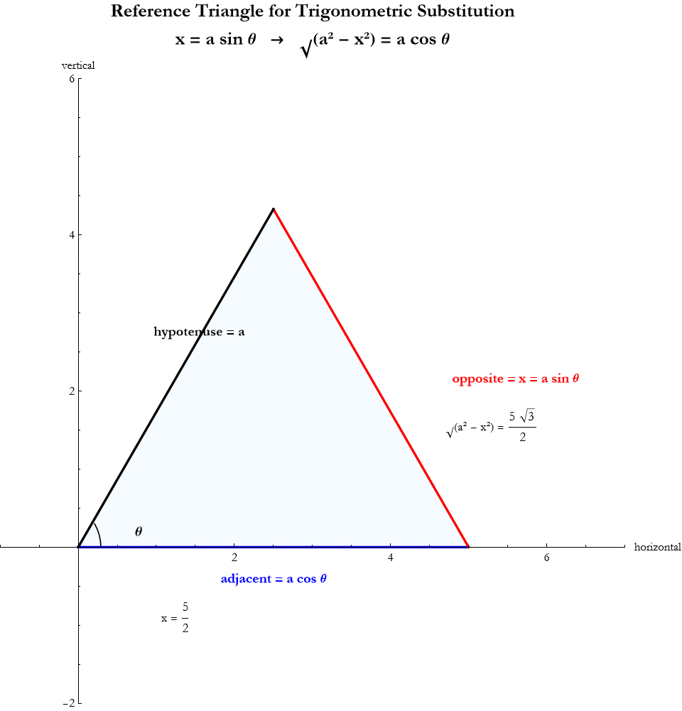
Definitions

Definition 24.31 Trigonometric Substitution: Replacing the variable x with a trigonometric expression to simplify a square root of a quadratic.

Definition 24.32 Reference Triangle: A right triangle constructed from the substitution to express θ back in terms of x.

Principles

Principle 24.50: Match the substitution to the quadratic form under the square root. This works because it exploits the Pythagorean identity to eliminate square roots.

Principle 24.51: The method trades algebraic complexity for trigonometric simplicity.

Exercise 24.82: Begin with Algorithm 24.10. Copy this into your notebook. Reflect on its meaning for a few minutes. Note any thoughts that come to mind. How would you explain this to someone sitting in front of you. Write this down. Do this for each definition and principle.

Exercise 24.83: Use trigonometric substitution to evaluate .

Exercise 24.84: Compute using the tangent substitution. Draw the reference triangle.

Exercise 24.85: Evaluate .

Exercise 24.86: Find using the secant substitution.

Exercise 24.87: The arc length of the curve (upper half of an ellipse) involves . Set up the integral using trigonometric substitution but do not evaluate it.

Exercise 24.88: Why do trigonometric substitutions appear so frequently in physics problems involving circles, ellipses, and hyperbolas? What deeper geometric connection is at work?

Hyperbolic Integrals

You have already mastered trigonometric substitution and trigonometric integrals. Now we turn to their close relatives, the hyperbolic functions. These functions—sinh, cosh, tanh, and their inverses—arise naturally whenever exponential growth or decay is involved. They simplify many integrals that contain square roots of the form or , and they appear in important physical problems.Hyperbolic integrals are often cleaner and more natural than their trigonometric counterparts for these situations.

Case 1: ∫sinh⁡ x dx=cosh ⁡x+c

Case 2: ∫cosh ⁡x dx=sinh ⁡x+c

Case 3: Integrals involving .

These are best handled by hyperbolic substitution (the hyperbolic analogue of trigonometric substitution):

For we let x=a sinh u.

For we let x=a cosh⁡ u.

Look for expressions of the form or powers/products of hyperbolic functions.

Use the substitution suggested by the quadratic form (sinh for + , cosh for – ).

Simplify using the identity .

Integrate with respect to the new variable u.

Convert back to x using or , or express in logarithms.

Definition

Definition 24.33 Hyperbolic Integral: An integral whose integrand involves hyperbolic functions or can be simplified by hyperbolic substitution .  

Exercise 24.89: Begin with Algorithm 24.11. Copy this into your notebook. Reflect on its meaning for a few minutes. Note any thoughts that come to mind. How would you explain this to someone sitting in front of you. Write this down. Do this for each definition and principle.

Exercise 24.90: Use the substitution x=a sinh u to compute .

Exercise 24.91: The catenary curve (shape of a hanging chain) has equation y=a cosh⁡(x/a). Set up the arc-length integral and simplify it using hyperbolic identities.

Exercise 24.92: Show that can be evaluated using hyperbolic definitions (for a>∣b∣).

The Rationalizing Substitution

Sometimes the square root refuses to yield to trigonometric or hyperbolic tricks. In those cases, a clever algebraic substitution that makes the radical itself the new variable can rationalize the entire expression and open the door to ordinary integration. You have now mastered trigonometric substitution and hyperbolic substitution—powerful geometric tools for integrals containing , , and . Yet there remains an important family of integrals where the radical is linear in the variable or appears in a form that resists those methods.

The rationalizing substitution (sometimes called the Euler substitution) is the technique that directly attacks the square root by setting it equal to a new variable. This removes the radical completely and turns the integrand into a rational function that can often be integrated using partial fractions or simple polynomials.

Use the rationalizing substitution when the integrand contains:

Expressions where a linear fractional transformation can eliminate the square root.

Let this implies that .

Solving for x we get and we get dx=2 t/a dt.

The square root disappears and the integrand becomes a rational function in t.

For example, if we want to compute

(24.128)

Let , so , dt=2 t dt. Then

(24.129)

We then back substitute,

(24.130)

Identify the radical (usually linear under the square root).

Set the entire square root equal to a new variable.

Solve for the original variable and its differential in terms of the new variable.

Substitute so the the radical vanishes.

Integrate.

Back substitute.

Definition

Definition 24.34 Rationalizing Substitution: A substitution in which the square root itself is set equal to a new variable, eliminating the radical from the integrand.

    Principles

Principle 24.57:  When a square root is linear, let the radical be the new variable.

Principle 24.58:  This method is especially powerful when the expression under the radical is linear.

Exercise 24.93: Begin with Algorithm 24.12. Copy this into your notebook. Reflect on its meaning for a few minutes. Note any thoughts that come to mind. How would you explain this to someone sitting in front of you. Write this down. Do this for each algorithm, definition and principle.

Exercise 24.94: Use rationalizing substitution to evaluate .

Exercise 24.95: Calculate .

Exercise 24.96: Evaluate .

Exercise 24.97: Set up the rationalizing substitution for and simplify the integrand.

Integration by Partial Fraction Expansion

You have now learned a powerful collection of integration techniques, substitution, integration by parts, trigonometric and hyperbolic substitutions, and rationalizing substitutions. Yet one of the most frequent and useful methods remains, the partial fraction expansion.

Many physical problems lead to rational functions—ratios of polynomials. These often look difficult to integrate directly. Partial fractions allow us to decompose such a function into a sum of simpler fractions, each of which can be integrated using techniques you already know.

Use partial fraction decomposition when the integrand is a proper rational function—that is, the degree of the numerator is less than the degree of the denominator. (If it is not proper, first perform polynomial long division.)

Definition 24.35 Partial Fraction Expansion: The process of writing a rational function as a sum of simpler fractions whose denominators are the factors of the original denominator.

There are three cases:

Case 1 Distinct Linear Factors: If the denominator factors into distinct linear terms , write

(24.131)

Case 2 Repeated Linear Factors: For a repeated factor , include terms up to the power k

(24.132)

Case 3 Irreducible Quadratic Factors: For an irreducible quadratic , use

(24.133)

In RC circuits, we often encounter

(24.134)

We decompose this,

(24.135)

Solving this gives A=1 and B=-1, so

(24.136)

Algorithm 24.14 The General Method for Partial Fraction Expansion Integration

Check that the fraction is proper (or perform polynomial division first).

Factor the denominator completely.

Write the partial fraction decomposition with unknown constants.

Multiply both sides by the denominator and equate coefficients (or use convenient values of the variable).

Integrate each simple term separately.

    Principles

Principle 24.59: Partial fraction expansion turns a single complicated rational function into a sum of simpler fractions that are easy to integrate.

Principle 24.60: The method works because any rational function can be uniquely decomposed into partial fractions once the denominator is fully factored.

Exercise 24.98: Begin with Definition 24.65. Copy this into your notebook. Reflect on its meaning for a few minutes. Note any thoughts that come to mind. How would you explain this to someone sitting in front of you. Write this down. Do this for each algorithm, and principle.

Exercise 24.99: Decompose (3 x+2)/[(x-1)(x+3)] into partial fractons and integrate.

Exercise 24.100: Evaluate .

Exercise 24.101: Evaluate .

Exercise 24.102: Evaluate .

Numerical Integration

Not every integral we meet in physics has a nice closed-form antiderivative. When the function is complicated, the limits are awkward, or the problem is simply too realistic, we turn to numerical integration — the art of turning the definite integral back into a sum of many small pieces. You have now learned a wide array of analytic techniques—substitution, integration by parts, trigonometric and hyperbolic substitutions, partial fractions, and more. These methods serve you beautifully when the integral yields to them. Yet in real theoretical physics, many integrals refuse to surrender an elegant antiderivative. The force law may be complicated, the geometry irregular, or the problem may involve data from experiment rather than a clean formula.

Numerical integration is the powerful practical art of computing definite integrals by turning them back into sums—exactly the idea that gave birth to the definite integral in the first place. It lets you obtain accurate numerical answers even when symbolic methods fail.

Definition 24.28 Numerical Integration (Quadrature): Any method that approximates the definite integral

(24.137)

by a weighted sum of function values at carefully chosen points.There are many ways of doing this. We explore two.

Trapezoidal Rule: Divide [a, b] into n subintervals of width w=(b−a)/n. Then

(24.138)

Simpson’s Rule (More Accurate): For an even number of subintervals,

(24.139)

Simpson’s rule is remarkably accurate for smooth functions and is often the default choice for moderate precision.

In practice, you will rarely write your own quadrature routines. Modern tools do this for you with high accuracy and adaptive step size

If you want to use the Trapezoidal Rule we write.

There are other options to play with, too. AccuracyGoal specifies the number of digits of accuracy we want. Accuracy is how close we want to be to the actual value. Precision goal specifies the digits of precision. Precision is how far we want to evaluate a calculation. You can be precisely inaccurate.

Here is an example.

To use Simpson’s rule we specify the Method “NewtonCotesRule”.

When we use numerical integration (Trapezoidal rule, Simpson’s rule, or NIntegrate), we replace the exact integral with a sum. This always introduces some error. A good physicist or mathematician learns not only how to compute the integral numerically, but also how to estimate, control, and interpret that error. A good physicist or mathematician learns not only how to compute the integral numerically, but also how to estimate, control, and interpret that error.

There are two main sources of error in numerical integration.

The first type we will consider is the error caused by the approximation itself, we call this truncation error. For one interval of the trapezoidal rule we have

(24.140)

For the entire rule with n subintervals w=(b-a)/n we have,

(24.141)

For Simpson’s rule we get

(24.142)

The precise methods for figuring out these errors is beyond our scope, at present. UsingNintegrate we can do the following workflow to estimate the truncation error.

For our example above we have

Note the extremely low error.

The second kind of error comes from the limited precision of computer arithmetic (floating-point numbers), we call this round-off errors. These are important only where the step size is extremely small, or the function values become very large or very small.

Definition

Definition 24.29 Adaptive Quadrature: Methods that automatically refine the grid where the function changes rapidly. In Wolfram Language use Method->”GlobalAdaptive” or Method->”LocalAdaptive”.

Principles

Principle 24.61: Numerical integration is not a last resort—it is a fundamental way of computing the definite integral when analytic methods are unavailable or impractical.

Principle 24.62: The accuracy of numerical integration depends on the smoothness of the function, the number of points used, and the cleverness of the quadrature rule.

Principle 24.63: In theoretical physics, we often combine analytic insight (to simplify the integrand) with numerical integration (to get the final number).

Principle 24.64: Always estimate the error. A good numerical result includes not just the value, but a sense of how trustworthy it is.

Principle 24.65: Every definite integral is ultimately a limit of sums—numerical methods simply take this limit practically.

Exercise 24.103: Begin with Definition 24.28. Copy this into your notebook. Reflect on its meaning for a few minutes. Note any thoughts that come to mind. How would you explain this to someone sitting in front of you. Write this down. Do this for each definition, and principle.

Exercise 24.104: Use the trapezoidal rule with n=4 and n=8 to approximate .

Exercise 24.105: Explain why Simpson’s rule usually gives much smaller error than the trapezoidal rule for the same number of intervals.

Exercise 24.106: Use NIntegrate with the PrecisionGoal and AccuracyGoal options to compute and request an error estimate.

Exercise 24.107: When is it better to spend time simplifying an integral analytically versus using a high-precision numerical method? Give examples from physics.

Summary

Write a summary of this lesson.

For Further Study

Jerrold E. Marsden, Alan Weinstein, (1985), Calculus II. Springer-Verlag, New York. You can download it for free from CalTech: https://www.cds.caltech.edu/~marsden/volume/Calculus

Silvanus Thompson, (1914), Calculus Made Easy. MacMillan and Co. Released by The Project Gutenberg in 2012. This book has inspired generations of physicists and engineers precisely because it removes fear and reveals beauty—exactly what you’re doing in your course. Many people who later tackle The Theoretical Minimum started with Thompson and say it gave them the courage to continue.

Paul J. Nahin, (2020), Inside Interesting Integrals, Springer. This is chock full of methods, and it goes far beyond where we are now. There is a less expensive book available through Kindle.

Marat V Markin, (2019), Integration for Calculus, Analysis, and Differential Equations. World Scientific Publishing Co. Pte. Ltd. This is a very nice book that goes into great detail about many of the topics in this lesson.

Seán M. Stewart, (2018), How to Integrate It, Cambridge University Press. This book expands the last two lectures to an entire book.

3Blue1Brown – Essence of Calculus, Chapter 8: Integration
Best visual intuition for the fundamental theorem and applications.
→ https://www.youtube.com/watch?v=rfG8ce4nNh0
Full playlist: https://www.youtube.com/playlist?list=PLZHQObOWTQDMsr9K-rj53DwVRMYO3t5Yr

Professor Leonard – Calculus 2: Integration Techniques
Thorough blackboard-style lectures.
→ Start here: https://www.youtube.com/watch?v=b2ZFpE_yrLg
Full playlist: Search “Professor Leonard Calculus 2” on YouTube.

Blackpenredpen – Integration Techniques Playlist
Excellent for tricky integrals and partial fractions.
→ https://www.youtube.com/playlist?list=PLj7p5eZf9p9g5fQfZfZfZfZfZfZfZfZfZ (look for Integration playlist)

Michel van Biezen – Calculus 2 Integration
Very clear and well-organized.
→ https://www.youtube.com/playlist?list=PLX2gQf3G8Yd4f5fQf3G8Yd4f5fQf3G8Yd