Lesson 23 Calculus 4 Integration in One Variable
“Integration is the art of finding the whole from its infinitesimal parts. It is the inverse of differentiation, and together they unlock the secrets of motion and growth.”—Gottfried Wilhelm Leibniz
“Integration is the friendliest operation in calculus. It turns rates into totals, slopes into areas, and tiny changes into meaningful quantities.”—Richard Feynman
Introduction
We have spent the previous lessons building a deep understanding of derivatives—the mathematics of instantaneous change. Now we turn to the second great pillar of calculus, that of integration. While differentiation breaks things down into rates, integration builds them back up—it is the mathematics of accumulation, of summing infinitesimal pieces to understand the whole.
The central idea of this lesson is this—integration reverses differentiation. It allows us to go from a rate of change (a derivative) back to the original quantity, and to calculate totals—total distance traveled, total work done, total energy stored, total mass, and total area—by adding up infinitely many tiny contributions. In physics, integration turns local information into global understanding.
This lesson marks a major turning point. You will learn not only how to compute integrals, but how to use them to solve real physical problems, finding the work done by a variable force, calculating kinetic energy, determining centers of mass, computing hydrostatic pressure, and laying the foundation for solving differential equations—one of the central problems in mathematical physics. Integration is where calculus becomes a truly powerful tool for describing the physical world.
As we work through the coming topics, you will see integration transform from an abstract summation process into a practical method for solving problems that derivatives alone cannot address. You will discover how the area under a curve can represent energy, how reversing a derivative recovers position from velocity, and how integration connects the infinitesimal to the measurable.You have already come far. Now, with integration, you gain the ability to accumulate change and reveal the full story hidden in rates. This is where calculus truly begins to show its power in theoretical physics.
Let us begin.
The Riemann Sum
We have learned how derivatives describe instantaneous rates of change. Now we turn to the complementary question, “How can we calculate the total accumulated change over an interval?” How do we find the total distance traveled from a velocity function, or the total work done by a variable force?
The answer begins with a simple but powerful idea—approximating areas under curves by summing rectangles. To find the area under a curve (or the accumulated quantity it represents), we divide the interval into many thin rectangles, compute the area of each, and add them up. As we make the rectangles narrower and narrower, this sum gets closer and closer to the true accumulated value. This approximation technique is called a Riemann sum.
Definition 23.1 The Riemann Sum: Let f(x) be a positive, continuous function on an interval [a, b]. Divide the interval into n subintervals, each of width
![]()
(23.1)
Choose a sample point ![]() in the ith subinterval. The area of the ith rectangle is
in the ith subinterval. The area of the ith rectangle is ![]() . The total approximate area is the Riemann sum
. The total approximate area is the Riemann sum
![]()
(23.2)
Different choices of ![]() give different sums:
give different sums:
Left Riemann sum: Use the left endpoint of each subinterval.
Right Riemann sum: Use the right endpoint.
Midpoint Riemann sum: Use the midpoint.
As n→∞ (and Δ x→0), the Riemann sum approaches the exact area under the curve.
The Riemann sum also has a direct physical meaning. If f(x) represents force as a function of displacement, the Riemann sum approximates the total work done. If f(t) is velocity as a function of time, it approximates the total distance traveled.
As an example, we approximate the area under ![]() from x=0 to x=3 using a right Riemann sum with n=6, and let Δ x=(3-0)/6=0.5, then
from x=0 to x=3 using a right Riemann sum with n=6, and let Δ x=(3-0)/6=0.5, then
![]()
(23.3)
When i=1, then ![]() . When i=2, then
. When i=2, then ![]() . When i=3, then
. When i=3, then ![]() . When i=4, then
. When i=4, then ![]() . When i=5, then
. When i=5, then ![]() . When i=6, then
. When i=6, then ![]() .
.
Then we add these up 0.125+0.5+1.125+2+3.125+4.5=11.375, while the exact area turns out to be 9 (as we will see later).
This gives an approximation of 9.6875 (the exact area is 9).
For a second example a car’s velocity is ![]() m/sec from t=0 to t=6 seconds. Using a midpoint Riemann sum with n=6, estimate the total distance traveled.
m/sec from t=0 to t=6 seconds. Using a midpoint Riemann sum with n=6, estimate the total distance traveled.
We divide the interval [0,6] into 6 subintervals, each was a width
![]()
(23.4)
The midpoint of the ith subinterval is ![]() , for i=1 to 6.
, for i=1 to 6.
The midpoints are: 0.5,1.5,2.5,3.5,4.5,5.5.
We now evaluate v(t) at each midpoint and multiply by Δ t=1. When t=0.5, then ![]() . When t=1.5, then
. When t=1.5, then ![]() . When t=2.5, then
. When t=2.5, then ![]() . When t=3.5, then
. When t=3.5, then ![]() . When t=4.5, then
. When t=4.5, then ![]() . And when t=5.5, then
. And when t=5.5, then ![]() .
.
The midpoint Riemann sum is the sum of these values (since Δ t=1), so we have 3.75+9.75+13.75+15.75+15.75+13.752=72.5 meters.
This approximation gives about 72 meters (exact value is 72 m as we will see later).
We can visualize this in Wolfram Language.
The Riemann sum is the bridge between discrete approximations and the continuous world of calculus. It prepares us for the definite integral—the limit that makes these approximations exact.
Definitions
Definition 23.2 Left Riemann Sum: A Riemann sum that uses the left endpoint of each subinterval as the sample point.
Definition 23.3 Right Riemann Sum: A Riemann sum that uses the right endpoint of each subinterval as the sample point.
Definition 23.4 Midpoint Riemann Sum: A Riemann sum that uses the midpoint of each subinterval as the sample point.
Principles
Principle 23.1 Approximation by Riemann Sums: The area under a curve (or any accumulated quantity it represents) can be approximated by summing the areas of thin rectangles. As the number of rectangles increases (n→∞) and their width Δ x→0, the Riemann sum approaches the exact accumulated value.
Exercise 23.1: Begin with Definition 23.1. Copy this into your notebook. Reflect on its meaning for a few minutes. Note any thoughts that come to mind. How would you explain this to someone sitting in front of you. Write this down. Do this for each definition and principle.
Exercise 23.2: Approximate the area under the curve f(x)=2x+1 from x=0 to x=4 using a right Riemann sum with n=4.
1) Compute Δ x and list the right endpoints.
2) Calculate each rectangle’s area and sum them to find the approximation.
Exercise 23.3: Use a midpoint Riemann sum with n=6 to approximate the area under ![]() from x=1 to x=4.
from x=1 to x=4.
1) Compute Δ x and list the midpoints.
2) Compute the full sum step by step.
3) How does this approximation compare to the left and right Riemann sums (in terms of over- or under-estimation)?
Exercise 23.4: A car’s velocity is given by ![]() m/sec from t=0 to t=6 seconds.
m/sec from t=0 to t=6 seconds.
1) Compute Δ x and list the right endpoints.
2) Calculate each rectangle’s area and sum them to find the approximation.
Exercise 23.5: Approximate the area under ![]() from x=1 to x=9 using right Riemann sums with n=4, n=8, and n=16.
from x=1 to x=9 using right Riemann sums with n=4, n=8, and n=16.
1) Calculate each approximation.
2) Observe the pattern as n increases.
Exercise 23.6:
1) Explain in your own words why the Riemann sum becomes more accurate as n increases and Δ x decreases.
2) Why is the Riemann sum a natural tool for calculating total distance from a velocity function or total work from a force function?
3) Give one physical situation (not from the exercises above) where you would use a Riemann sum to approximate a total accumulated quantity. What function would you sum?
The Definite Integral
We have seen how Riemann sums provide increasingly accurate approximations of accumulated quantities by summing many thin rectangles. Now we take the final, crucial step by letting the number of rectangles grow without bound and the width of each rectangle shrink to zero. What remains is one of the most important concepts in calculus. The definite integral is the exact limit of Riemann sums as the partition becomes infinitely fine. It represents the precise accumulated value of a quantity—the exact area under a curve, the total distance traveled, or the total work done by a variable force.
Definition 23.5 Definite Integral: Let f(x) be a continuous function on the closed interval [a, b]. The definite integral of f from a to b is defined as
![]()
(23.5)
This limit exists and is the same regardless of how we choose the sample points (left, right, or midpoint) when f is continuous. Note the we sometimes call the endpoints of the interval, we call them limits of integration.
The symbol ∫ is called Summa, and is an elongated “S” (for “sum”), and dx reminds us of the infinitesimal width of each rectangle in the limit.
If f(x) represents force as a function of displacement, then the definite integral is the total work done.
If f(t) represents velocity as a function of time, the definite integral is the total distance traveled (net displacement if velocity changes sign).
If f(x) represents density, the integral gives the total mass.
Let’s say that we want to compute
![]()
(23.5)
From this we see that we have the interval [0,3], we divide this into n subintervals
![]()
(23.6)
Using the right Riemann sum, the sample points are ![]() for i=1,2,...,n.
for i=1,2,...,n.
Then the Right Riemann Sum is
![]()
(23.7)
We note a formula for the sum of squares
![]()
(23.8)
so
![]()
(23.9)
Now we take the limit as n->∞,
![]()
(23.10)
Thus
![]()
(23.11)
For another example, a car’s velocity is ![]() m/sec from t=0 to t=6. The total distance traveled is
m/sec from t=0 to t=6. The total distance traveled is
![]()
(23.12)
Again we divide the interval into n subintervals
![]()
(23.13)
Using the right Riemann sum, the sample points are ![]() for i=1,2,...,n.
for i=1,2,...,n.
Then the Right Riemann Sum is
![]()
(23.14)
We simplify inside the square
![]()
(23.15)
We can split this into two sums.
![]()
(23.16)
We will use (23.9) and
![]()
(23.17)
We get,
![]()
(23.18)
We then take the limit as n->∞
![]()
(23.19)
Therefore,
![]()
(23.20)
The force on a spring is given by F(x)=k x, where k=200 N/m and x is the displacement from equilibrium. Compute the work done by the spring force when stretching the spring from x=0 to x=0.2 m by evaluating the definite integral
![]()
(23.21)
using the limit of Riemann sums.
Divide the interval [0, 0.2] into b subintervals, each of width
![]()
(23.22)
Using right Riemann sums, the sample points are ![]() for i=1,2,…,n.
for i=1,2,…,n.
The right Riemann sum for the work is
![]()
(23.23)
We then use (23.18)
![]()
(23.24)
We take the limit as n->∞
![]()
(23.25)
Therefore
![]()
(23.26)
We can see this sort of thing in Wolfram Language.
Reflect on how the definite integral is the natural limit of the summing process we studied in the previous section. The definite integral is the tool that turns the approximation method of Riemann sums into an exact mathematical operation. It is the counterpart to the derivative and the foundation for calculating accumulated physical quantities in theoretical physics.
We will return to this idea a little later.
Exercise 23.7: Evaluate the definite integral ![]() by interpreting it as the area under the curve.
by interpreting it as the area under the curve.
1) Sketch the region and compute the area geometrically (as a trapezoid).
2) Verify your result using the definition as the limit of Riemann sums (right endpoints, n=4).
3) Interpret the result physically if f(x)=3x+2 represents velocity in m/sec.
Exercise 23.8: A particle moves with velocity ![]() m/sec from t=0 to t=6 seconds.
m/sec from t=0 to t=6 seconds.
1) Write the definite integral that represents the total distance traveled.
2) Evaluate the integral.
3) Compare this to the midpoint Riemann sum approximation with n=6 from earlier work.
Exercise 23.9: The force acting on an object is ![]() newtons, where x is displacement in meters.
newtons, where x is displacement in meters.
1) Write the definite integral that represents the work done from x=0 to x=3 m.
2) Evaluate the integral.
3) Interpret the sign and magnitude of the result physically.
Exercise 23.10: Use Wolfram Language to evaluate the following definite integrals:
1) ![]() . Plot the integrand and shade the region under the curve.
. Plot the integrand and shade the region under the curve.
2) ![]() .
.
Exercise 23.11: The velocity of a falling object (ignoring air resistance) is v(t)=9.8t m/sec, starting from rest at t=0.
1) Write the definite integral that gives the distance fallen from t=0 to t=5 seconds.
2) Evaluate the integral.
3) Explain what the definite integral physically represents in this context.
Exercise 23.12:
1) Explain in your own words the difference between a Riemann sum and the definite integral.
2) Why is the definite integral a natural tool for calculating total distance, total work, or total mass?
3) Give one real-world physical situation (not from the exercises above) where the definite integral would be used to find an accumulated quantity. What function would you integrate, and what would the result represent?
Antiderivatives
We have seen how the definite integral accumulates change over an interval. Now we ask the natural reverse question, “Given a rate of change (a derivative), can we recover the original quantity?” This brings us to one of the most important ideas in calculus An antiderivative of a function f(x) is another function F(x) whose derivative is f(x). In other words, antiderivatives reverse the process of differentiation. They allow us to go from a known rate of change back to the original quantity—from velocity to position, from acceleration to velocity, or from force to potential energy.
Definition 23.6 Antiderivative: A function F(x) is called an antiderivative of f(x) if F'(x)=f(x). We sometimes call F(x) a primitive function.
If we know the derivative of a function, we can work backwards to find possible original functions. For example, if the derivative is 2 x, then an antiderivative is ![]() (because the derivative of
(because the derivative of ![]() is 2 x). If the derivative is
is 2 x). If the derivative is ![]() , then an antiderivative is
, then an antiderivative is ![]() (because the derivative of
(because the derivative of ![]() is
is ![]() ).
).
This reverse process is not always unique—different functions can have the same derivative (they differ by a constant)—but the pattern is powerful and consistent.
Suppose the derivative of a function is ![]() . What could the original function f(x) be? By working backwards term by term
. What could the original function f(x) be? By working backwards term by term
![]()
(23.28)
(You can check by differentiating this result to recover the original derivative.)
As another example the velocity of a particle is given by v(t)=9.8t m/sec (free fall under gravity, starting from rest). Find a possible position function s(t). Working backwards from velocity
![]()
(23.29)
If the particle starts at position s(0)=0, this function satisfies the condition perfectly.
For another example, the force on a spring is F(x)=−k x. A possible potential energy function U(x) satisfies F(x)=−dU/dx, so working backwards
![]()
(23.30)
This is the familiar elastic potential energy stored in a stretched or compressed spring.
We can compare the curves in Wolfram Language.
How does finding antiderivatives connect to recovering position from velocity or potential energy from force in physical systems?Antiderivatives are the inverse operation to differentiation. They allow us to reconstruct quantities from their rates of change—a skill that becomes essential when we study the Fundamental Theorem of Calculus and apply integration to real physical problems.
Theorems
Theorem 23.1 Constant Rule: The antiderivative of a constant is the product of the constant and the relevant variable.
![]()
(23.31)
Proof of Theorem 23.1: This is a direct proof. By definition, the derivative of F(x) at any point x is
![]()
(23.32)
provided the limit exists.
Substitute F(x)=k x
![]()
(23.33)
So the difference quotient becomes
![]()
(23.34)
This expression equals k for every Δ x≠0. Therefore,
![]()
(23.35)
Hence, F'(x)=k for all x, which means F(x)=k x is indeed an antiderivative of the constant function f(x)=k. QED
Theorem 23.2 Power Rule:
![]()
(23.36)
Proof of Theorem 23.2: This is a direct proof. By definition,
![]()
(23.37)
Substitute
![]()
(23.38)
Then
![]()
(23.39)
The difference quotient is
![]()
(23.40)
Now expand ![]() using the Binomial Theorem (see Lesson 20)
using the Binomial Theorem (see Lesson 20)
![]()
(23.41)
Then
![]()
(23.42)
Then
![]()
(23.43)
Then
![]()
(23.44)
Now take the limit
![]()
(23.45)
Note that every term containing a positive power of Δ x goes to zero. Therefore,
![]()
(23.46)
this shows that ![]() is indeed an antiderivative of
is indeed an antiderivative of ![]() . QED
. QED
Theorem 23.3 Sine Rule:
![]()
(23.47)
Proof of Theorem 23.3: This is a direct proof. By definition,
![]()
(23.48)
Substitute F(x)=−cos x, then
![]()
(23.49)
The difference quotient becomes
![]()
(23.50)
We now use the trigonometric identity for the difference of cosines (see Lesson 15),
![]()
(23.51)
So
![]()
(23.52)
Rewrite the fraction
![]()
(23.53)
Thus the difference quotient is
![]()
(23.54)
Now take the limit, where as Δ x->0 then x+Δ x/2->x so sin (x+Δ x/2)->sin x. Then
![]()
(23.55)
Hence, F'(x)=sin x, which shows that F(x)=−cos x is an antiderivative of sin x. QED
Theorem 23.4 Cosine Rule:
![]()
(23.56)
Exercise 23.13: Prove Theorem 23.4
Theorem 23.5 Polynomial Rule: For a polynomial and antiderivative is obtained term by term using the power rule.
Exercise 23.14: Prove Theorem 23.5
Exercise 23.15: Begin with Definition 23.6. Copy this into your notebook. Reflect on its meaning for a few minutes. Note any thoughts that come to mind. How would you explain this to someone sitting in front of you. Write this down. Do this for each definition, theorem, and proof.
Exercise 23.16: Find an antiderivative for each of the following functions:
1) f(x)=7.
2) ![]() .
.
3) ![]()
4) ![]()
Exercise 23.17: For each pair, verify by direct differentiation that the second function is an antiderivative of the first:
1) ![]() .
.
2) f(x)=sin x,F(x)=−cos x.
3) ![]() .
.
Exercise 23.18: A particle moves along a straight line with velocity ![]() m/sec. Find a function s(t) (an antiderivative of v(t)) that gives the position of the particle. What does the constant term in your answer physically represent?
m/sec. Find a function s(t) (an antiderivative of v(t)) that gives the position of the particle. What does the constant term in your answer physically represent?
Exercise 23.19: The force on a spring is given by F(x)=−k x, where k>0 is the spring constant and x is the displacement from equilibrium. Find a function U(x) that is an antiderivative of −F(x). Show that this U(x) has the familiar form of elastic potential energy.
Exercise 23.20: Find an antiderivative for each of the following functions:
1) ![]()
2) ![]() .
.
3) ![]()
Exercise 23.21:
1) Define in Wolfram Language:
f[x_] := 6 x^2 - 4 x + 5;
F[x_] := 2 x^3 - 2 x^2 + 5 x;
Verify that D[F[x], x] equals f[x].
2) Plot both f(x) and F(x) on the same graph from x=−2 to x=3. Describe the relationship you observe between the two curves.
3) Experiment: Change the constant term in F(x) (add +3 or -7) and re-plot. What happens to the derivative?
Properties of Definite Integrals
Once we define the definite integral as the net accumulated change (or signed area) under a curve, certain predictable behaviors emerge naturally from the way we add up small pieces. These properties let us simplify complicated integrals, exploit symmetry, change variables in a controlled way, and break big problems into smaller ones—all without actually computing the integral yet. They are powerful algebraic tools that make integration far more practical.
We now have two seemingly different ideas, the definite integral (which accumulates signed area or total change by adding up many tiny pieces) and the antiderivative (which recovers an original quantity from its rate of change). This section reveals that these two concepts are intimately connected. In fact, they are inverse operations. The definite integral from a to b of a function f is exactly the difference in the values of any antiderivative of f evaluated at the endpoints. This single theorem turns the hard work of summing infinitely many pieces into a simple subtraction—one of the most powerful shortcuts in all of mathematics and theoretical physics.
Theorem 23.5 The Fundamental Theorem of Calculus, Part I: Let f be a continuous function on the closed interval [a, b]. Let F be any antiderivative of f, that is, F'(x)=f(x) for all x in the closed interval. Then
![]()
(23.57)
The definite integral accumulates tiny changes from a to b. An antiderivative F(x) tracks the total accumulated quantity whose rate of change is f(x). The Fundamental Theorem says these two processes are inverses, thus to find the net accumulated change, simply evaluate the antiderivative at the upper limit and subtract its value at the lower limit. This turns an infinite sum into ordinary subtraction. I will present a proof of this later.
Theorem 23.6 Zero Integral (Same Limits):
![]()
(23.58)
Exercise 23.22: Prove Theorem 23.6.
Theorem 23.7 Reversing Limits:
![]()
(23.59)
Proof of Theorem 23.7: This is a direct proof. Assume first that a<b. For ![]() we begin by partitioning the interval [a, b] into n subintervals, each of width
we begin by partitioning the interval [a, b] into n subintervals, each of width
![]()
(23.60)
A general Riemann sum is
![]()
(23.61)
where ![]() is a sample point in the ith subinterval. Taking the limit as n→∞
is a sample point in the ith subinterval. Taking the limit as n→∞
![]()
(23.62)
For ![]() we now partition the interval [b, a]. The same division points are used, but we travel from b down to a. The width of each subinterval is now
we now partition the interval [b, a]. The same division points are used, but we travel from b down to a. The width of each subinterval is now
![]()
(23.63)
The sample points ![]() are the same, but every width has flipped sign. Therefore the Riemann sum becomes
are the same, but every width has flipped sign. Therefore the Riemann sum becomes
![]()
(23.64)
Taking the limit as n→∞,
![]()
(23.65)
Thus,
![]()
(23.66)
There are two special cases:
If a=b, both sides are zero (by the zero integral property).
If a>b, the roles are simply swapped, and the same sign-flip argument applies.
QED
Theorem 23.8 Constant Multiple Rule:
![]()
(23.67)
Exercise 23.23: Prove Theorem 23.8.
Theorem 23.9 Linearity (Sum Rule):
![]()
(23.68)
Proof of Theorem 23.9: This is a direct proof. Consider a partition of the interval [a, b] into n subintervals, each of width Δ x=(b−a)/n. Let ![]() be any sample point in the ith subinterval.
be any sample point in the ith subinterval.
The Riemann sum for the sum function is
![]()
(23.69)
By the distributive property of multiplication over addition, this splits immediately into
![]()
(23.70)
where ![]() is the Riemann sum for f and
is the Riemann sum for f and ![]() is the Riemann sum for g.
is the Riemann sum for g.
Now take the limit as n→∞
![]()
(23.71)
Because the limit of a sum is the sum of the limits (provided each limit exists), we have
![]()
(23.72)
QED
Theorem 23.10 Additivity (Subdividing the Interval):
![]()
(23.73)
Exercise 23.24: Prove Theorem 23.10.
Theorem 23.11 Even and Odd Functions over Symmetric Limits:
Let the limits be symmetric about zero. If f is even (f(−x)=f(x)), then
![]()
(23.74)
If f is odd (f(−x)=−f(x)), then
![]()
(23.75)
Proof of Theorem 23.11: This is a direct proof by cases. We split the integral at zero using additivity
![]()
(23.76)
Case 1: Even Function
In the first integral, make the substitution u=−x. Then du=−dx.
When x=−a, u=a; when x=0, u=0. So
![]()
(23.77)
Since f is even, f(−u)=f(u), therefore
![]()
(23.78)
Adding the two pieces, we get
![]()
(23.79)
Case 2: Odd Function
Using the same substitution
![]()
(23.80)
Since f is odd, f(−u)=−f(u), so
![]()
(23.81)
Adding the two pieces, we get
![]()
(23.82)
QED
Theorem 23.12 Shifting the Limits (Translation):
For any constant k,
![]()
(23.83)
Exercise 23.25: Prove Theorem 23.12.
Theorem 23.13 Scaling the Limits:
For any constant c≠0,
![]()
(23.84)
(This is the change-of-variable formula in disguise and is extremely useful for simplifying integrals.)
Proof for Theorem 23.13: This is a direct proof by cases.
Case 1: c>0
Use the substitution
![]()
(23.85)
When x=a, , u=c a. When x=b, u=c b.
Substitute into the left-hand side
![]()
(23.86)
This is exactly the right-hand side. Done.
Case 2: c<0
Let c=−∣c∣ where ∣c∣>0. The substitution u=c x now reverses the direction of integration (the lower limit becomes larger than the upper limit).
The differential becomes dx=du/c. Because c<0, the factor 1/c is negative. By the Reversing Limits Theorem,
![]()
(23.87)
When we combine the negative sign from reversing limits with the negative 1/c, the two negatives cancel, and we again obtain
![]()
(23.88)
Thus the theorem holds for both positive and negative c. QED
Proof of Theorem 23.5: This is a direct proof. We prove this in two main steps.
Step 1: Define an auxiliary function and show it is also an antiderivative of f.
Define
![]()
(23.89)
for x in [a, b]. (This is the definite integral from the fixed lower limit a up to the variable upper limit x.)
We claim that G'(x)=f(x).
By the definition of the derivative,
![]()
(23.90)
Using the additivity property of definite integrals (Theorem 23.9), this simplifies to
![]()
(23.91)
Because f is continuous on the closed interval, it is bounded and attains its minimum and maximum values on any small subinterval. By the Extreme Value Theorem, there exists some number ![]() between x and x+Δ x such that
between x and x+Δ x such that
![]()
(23.92)
Therefore,
![]()
(23.93)
As Δ x→0, ![]() (because
(because ![]() is squeezed between x and x+h). By continuity the of f,
is squeezed between x and x+h). By continuity the of f,
![]()
(23.94)
Thus,
![]()
(23.95)
So G(x) is an antiderivative of f(x).
Step 2: Compare the two antiderivatives G and F.
Both G and F are antiderivatives of the same function f. Therefore, they differ by a constant G(x) = F(x) + C for some constant C, for allx in [a, b].
We evaluate at x = a,
![]()
(23.96)
Thus,
![]()
(23.97)
Now evaluate at x=b,
![]()
(23.98)
This is exactly the statement of the theorem. QED
For example,
![]()
(23.99)
As another example we will evaluate
![]()
(23.100)
in two ways. An antiderivative is ![]() , so
, so
![]()
(23.101)
Now we apply reversal,
![]()
(23.102)
Both give the same result.
In another example,
![]()
(23.103)
Let’s try a physics example, where the velocity of a particle is v(t)=6t−4 m/sec. Find the total distance traveled from t=1 to t=5 seconds. Using additivity at t=3
![]()
(23.104)
Solving the first term
![]()
(23.105)
Then the second term is
![]()
(23.106)
The total displacement = 16 + 40 = 56 meters.
Exercise 23.26: Begin with Theorem 23.5. Copy this into your notebook. Reflect on its meaning for a few minutes. Note any thoughts that come to mind. How would you explain this to someone sitting in front of you. Write this down. Do this for each theorem, and proof.
Exercise 23.27: Evaluate the definite integrals without using antiderivatives:
1) ![]() .
.
2) ![]() .
.
3) ![]() .
.
4) ![]() .
.
Exercise 23.28: Split the integral at x=2 and use linearity
![]()
Write the two separate integrals explicitly. Then explain why this splitting is useful even before computing the values.
Exercise 23.29: Evaluate the definite integrals using the fundamental theorem:
1) ![]() .
.
2) ![]() .
.
3) ![]() .
.
Exercise 23.30: A particle moves with velocity v(t)=10t−4 m/sec from t=1 to t=4 seconds.
1) Find the net displacement using the fundamental theorem.
2) Split the interval at t=2 using additivity and verify you get the same answer.
3) If this velocity came from a force F(x)=12x on a spring, interpret the sign of the work done from x=1 to x=3.
Exercise 23.31:
1) Show that ![]() .
.
2) Use scaling with c=2 to transform ![]() into an integral from 0 to 1. Write the exact new integral.
into an integral from 0 to 1. Write the exact new integral.
3) Combine symmetry and scaling to evaluate ![]() efficiently.
efficiently.
Indefinite Integrals
We have seen that the definite integral gives a specific number—the net accumulated change between two fixed limits. But what if we want the general antiderivative, the entire family of functions whose derivative is a given f(x)? This is the indefinite integral. It reverses differentiation completely, producing not one function but a whole class of functions that differ by an arbitrary constant. While incredibly useful, this generality creates practical headaches with notation and tables—issues we must face honestly if we are to use indefinite integrals responsibly in theoretical physics.
Definition 23.7 Indefinite Integral: The indefinite integral of a function f(x) is the set of all antiderivatives of f. It is written
![]()
(23.107)
where F(x) is any particular antiderivative of f(x) (so F'(x)=f(x)) and c is an arbitrary constant called the constant of integration. The symbol ∫f(x)dx does not represent a single function, instead it represents a whole family of functions that differ only by a constant.
In practice indefinite integrals cause two major practical difficulties
Notation suggests a single answer when there are infinitely many. The expression ![]() looks like “the” answer, yet every different value of c gives a different function. Tables of integrals almost always omit the +c, and this can mislead beginners into thinking the result is unique.
looks like “the” answer, yet every different value of c gives a different function. Tables of integrals almost always omit the +c, and this can mislead beginners into thinking the result is unique.
Tables and software often hide the constant as we will see in the next section. This is convenient for computation but hides the fact that the true general solution includes the arbitrary constant. In physics, forgetting the constant of integration can lead to incorrect solutions.
Because of these issues, many careful authors prefer to work with definite integrals whenever possible and introduce the indefinite integral mainly as a convenient shorthand for “find an antiderivative.”
The Fundamental Theorem of Calculus, Part I tells us that if we have a definite integral with limits, the arbitrary constant cancels out
![]()
(23.108)
The constant of integration disappears when we evaluate at two points. This is why definite integrals are cleaner and more physically meaningful.
Here are some examples,
![]()
(23.109)
![]()
(23.110)
![]()
(23.111)
Given velocity ![]() , the general position function is
, the general position function is
![]()
(23.112)
Here the constant constant of integration represents the initial position ![]() . Different values of c correspond to different starting points.
. Different values of c correspond to different starting points.
Table 23.1 Common Indefinite Integrals
| Function f(x) | Indefinite Integral | Notes |
| k | c+k x | Constant Rule |
| Power Rule | ||
| sin(x) | c-cos(x) | Sine Rule |
| cos(x) | c+sin(x) | Cosine Rule |
| c+tan(x) | Derivative of tan x | |
| Exponential Rule (k ≠ 0) | ||
| log({x})+c | Logarithmic Rule | |
| k f(x) | k×∫f[x]dx | Constant Multiple |
| f(x)+g(x) | ∫f[x]dx+∫g[x]dx | Linearity |
Table 23.2 Common Pitfalls with Indefinite Integrals
| Issue | What Happens | Why It Matters in Physics |
| Forgetting + c | You obtain only one particular antiderivative | Wrong initial or boundary conditions (position, energy, velocity, etc.) |
| Tables / software omit + c | Output appears as a single definite answer | Easy to forget the general family of solutions |
| Notation ∫f(x) dx | Looks like it represents one unique function | Can mislead students about the true nature of the result |
| Evaluating definite integrals | + c cancels automatically | This is why definite integrals are cleaner and safer in physics |
Principles
Principle 23.2 Families of Antiderivatives: An indefinite integral does not represent a single function. It represents an entire family of functions that differ only by a constant.
Principle 23.3 Notational Caution: The notation ∫f(x) dx is a convenient shorthand meaning “find an antiderivative of f(x),” but it can be misleading because it looks like it denotes one unique function. Tables and software frequently omit the + c, and that hides the true generality of the result.
Principle 23.4 Definite vs. Indefinite: When definite limits are present, the arbitrary constant of integration always cancels out. This is why definite integrals are cleaner and more physically meaningful than indefinite integrals.
Principle 23.5 Role of the Constant in Physics: In physical problems the constant of integration often carries real meaning—initial position, initial energy, reference point for potential energy, etc. Forgetting it can lead to incorrect or incomplete solutions.
Because indefinite integrals represent families of functions rather than single answers, many careful authors prefer to work with definite integrals whenever possible. The indefinite integral is most useful as a tool for finding antiderivatives before applying the Fundamental Theorem of Calculus.
Exercise 23.32: Begin with Definition 23.7. Copy this into your notebook. Reflect on its meaning for a few minutes. Note any thoughts that come to mind. How would you explain this to someone sitting in front of you. Write this down. Do this for each common indefinite integral, common pitfall, and principle.
Exercise 23.33: Find the indefinite integral:
1) f(x)=9
2) ![]()
3) ![]()
4) f(x)=sin x+cos x
Did you remember to include the constant of integration?
Exercise 23.34: For each pair, verify by direct differentiation that the second expression is the indefinite integral of the first:
1) ![]()
2) sin x,−cosx+n
3) ![]()
Exercise 23.35: A particle has velocity ![]() m/sec.
m/sec.
1) Find the general position function.
2) What does the constant of integration physically represent?
3) If the particle is at position s(0)=4 meters at t=0, find the specific position function.
Exercise 23.36: The force on a particle is F(x)=−12x+4. Find the general potential energy function U(x) such that F(x)=−dU/dx. Include the constant of integration and explain its physical meaning.
Exercise 23.37: Find the indefinite integral:
1) ![]()
2) ∫(4 sin x-2 cos x) dx
3) ![]()
Integrate[]
We have learned how to find antiderivatives by hand and how the Fundamental Theorem of Calculus connects them to definite integrals. Now we turn to the powerful Wolfram Language command Integrate[], which automates this process. It can compute both indefinite integrals (returning a family of antiderivatives) and definite integrals (returning a specific number). Understanding exactly what Integrate[] returns—especially how it handles the arbitrary constant—is essential for using it correctly in theoretical physics.
When you call Integrate[f[x], x], Wolfram Language returns one particular antiderivative. It does not automatically include the +c.
When you use the form Integrate[f[x], {x, a, b}], the command evaluates the definite integral directly using the Fundamental Theorem of Calculus (or advanced algorithms) and returns a specific numerical or symbolic value. The arbitrary constant cancels out automatically.
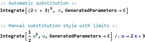
When you use the form Integrate[f[x], x,GeneratedParameters→C] the command evaluates the indefinite integral.
Here are some examples:
![]()
![]()
(Note: This is an antiderivative, no constant of integration is shown. You must remember to add it when working with indefinite integrals.)
![]()
![]()
This is also an antiderivative.
![]()
![]()
We now try a physics example.

![]()
![]()
The second command gives the exact net change in position without needing to add or subtract constants manually.
Exercise 23.38: Use Integrate[] to find the following:
1) Integrate[8 x^3 - 5 x^2 + 7, x]
2) Integrate[Sin[3 x] + Cos[2 x], x]
3) Integrate[E^(2 x), x]
Exercise 23.39: Compute each definite integral using Integrate[] with the {x, a, b} form:
1) ![]()
2) ![]()
3) ![]()
Exercise 23.40: A particle has velocity ![]() m/sec.
m/sec.
1) Use Integrate[v[t], t, GeneratedParameters -> C] to find the general position function
2) Use Integrate[v[t], {t, 1, 5}] to find the net displacement from t=1 to t=5 seconds.
3) Explain the physical meaning of the constant generated by Wolfram Language.
Exercise 23.41: For each function below, computer the indefinite integral b y hand (include +c), check the answer using Integrate[]. Differentiate with Wolfram Language to verify.
1) ![]()
2) 3 sin (2x)+5 cos x
Exercise 23.42: Run the following in Wolfram Language:
Integrate[x^2 + Sin[x], x, GeneratedParameters -> C]
Integrate[Integrate[x^2, x], x, GeneratedParameters -> C]
1) What constants does WL generate?
2) How many arbitrary constants appear after two integrations? Why?
3) Write the full general solution including all constants.
Exercise 23.40:
1) Compute both Integrate[4 x^3 - 2 x, x] and the corresponding definite integral from 1 to 3.
2) Explain why the definite integral result does not require adding a constant, while the indefinite one does.
3) When solving a physics problem (e.g., finding position from acceleration), which form of Integrate[] would you prefer to use first, and why?
4) What is the danger of forgetting to add +c (or the generated constants) when working with indefinite integrals?
Derivatives and Integrals as Operators
We have now seen derivatives and integrals from several angles—as rates of change, as accumulators of change, and as computational tools. We can go further and view both as rules that act on functions. One rule takes a function and produces its instantaneous rate of change. The other rule takes a function and produces its accumulated total change. These two rules are almost perfect inverses of each other—like forward and reverse operations—except for one small but important detail involving an arbitrary constant.
Definition 23.8 Operator: An operator is a rule that accepts a function as input and returns a new function as output. The derivative operator is written in several forms ![]() or d/dx or D[ , x] in Wolfram Language. The indefinite integral operator is written ∫… dx or Integrate[ , x, GeneratedParameters->C].
or d/dx or D[ , x] in Wolfram Language. The indefinite integral operator is written ∫… dx or Integrate[ , x, GeneratedParameters->C].
Principle 23.6 Inverse Relationship of Operators: Applying the integral operator and then the derivative operator (or vice versa) nearly returns the original function
![]()
(23.113)
![]()
(23.114)
Where the extra constant c appears because integration always produces a whole family of functions.
Principle 23.7 Linearity of Both Operators: Both the derivative and the integral are linear operators. For any constants a and b,
![]()
(23.115)
![]()
(23.116)
This linearity is why we can differentiate or integrate term by term.
Here we see this at work.

![]()
![]()
Here we reverse the process.

![]()
![]()
Let acceleration be constant: a(t)=−9.8 ![]() .
.
![]()
You will see two generated constants, which represent initial velocity and initial position.
![]()
![]()
![]()
![]()
Exercise 23.41: Begin with Definition 23.8. Copy this into your notebook. Reflect on its meaning for a few minutes. Note any thoughts that come to mind. How would you explain this to someone sitting in front of you. Write this down. Do this for each principle.
Exercise 23.42: Let ![]() .
.
1) Use Integrate[f[x], x] to find a particular antiderivative.
2) Apply the derivative operator D[ , x] to the result.
3) What do you recover? Does it match the original f(x)? Explain why this happens.
Exercise 23.43: Let ![]() .
.
1) Compute the derivative using D[g[x], x].
2) Integrate the result using Integrate[ , x].
3) How does the final expression compare to the original g(x)? What is the role of the constant that appears?
Exercise 23.44: Consider the functions ![]() and g(x) = sin x.
and g(x) = sin x.
1) Verify linearity of the derivative operator by hand and with D[], d/dx[3f(x)−2g(x)]=?
2) Verify linearity of the integral operator ∫[3f(x)−2g(x)] dx=? (include +c).
3) Explain why both operators being linear is useful in physics.
Exercise 23.45: A particle has constant acceleration a(t)=−9.8 ![]() .
.
1) Use Integrate[] twice (with GeneratedParameters -> C) to find the general velocity v(t) and position s(t).
2) How many arbitrary constants appear? What does each constant physically represent?
3) If you know v(0)=5 m/sec and s(0)=10 m, determine the specific functions.
Exercise 23.46: For ![]() :
:
1) Compute the derivative of the integral.
2) Compute the integral of the derivative.
3) Compare the two results and explain the difference you observe.
Riemann Integrability, Uniform Continuity, and Compactness (An Introduction to Real Analysis)
Not every function can be integrated using the Riemann approach. Some functions behave so erratically that no matter how finely we divide the interval, the upper and lower sums refuse to approach the same value. A function is Riemann integrable when those upper and lower sums get arbitrarily close as the partition becomes finer. This concept tells us precisely which functions we can safely integrate with the tools we have developed.
Definition 23.9 Partition of an Interval: A way of dividing an interval into subintervals. Each partition can be symbolized with P.
Definition 23.10 Norm (or Mesh) of a Partition: The length of the longest subinterval, denoted ||P||. When this value goes to 0 we are choosing to make the subintervals (the rectangles) infinitely thin.
Definition 23.11 Upper Riemann Sum (U(f,P)): Using the maximum value of f in each subinterval.
Definition 23.12 Lower Riemann Sum (L(f,P)): Using the minimum value of f in each subinterval.
Definition 23.13 Riemann Integrable: A bounded function f on a closed interval [a, b] is Riemann integrable if the upper and lower Riemann sums can be made arbitrarily close by choosing a sufficiently fine partition. That is, there exists a number I such that
![]()
(23.117)
This elegant statement means that no matter how we refine the partition, the pessimistic (upper) and optimistic (lower) estimates of the area under the curve get arbitrarily close to each other. Their common limit I is the definite integral.
Theorem 23.6 Continuous Functions Are Riemann Integrable: If f is continuous on the closed interval [a, b], then f is Riemann integrable on [a, b].
To prove this theorem we need a new concept. As we introduced in Lesson 18, ordinary continuity (or pointwise continuity) says that at each individual point, the function doesn’t jump—if you stay close enough to that point, the function values stay close together. Uniform continuity is stronger, the same “how close is close enough” works everywhere across the entire interval at once. There is one single δ that works for the whole domain, no matter where you are. This global control is what makes many powerful theorems (including the proof that continuous functions are Riemann integrable) possible.
Definition 23.14 Uniform Continuity: A function f is uniformly continuous on a set S if for every ε>0, there exists a δ>0 (depending only on ε, not on any particular point) such that for all x,y∈S,
![]()
(23.118)
In other words, no matter where you pick two points in S, as long as they are within δ of each other, their function values will be within ε of each other.
Theorem 23.7 Heine-Cantor Theorem: If f is continuous on the compact interval [a, b], it is uniformly continuous.
To prove this theorem we need to delve into some interesting properties of sets. Some intervals are “well-behaved”—they are finite in length and include their endpoints. These special intervals have powerful properties that make them extremely useful in analysis and theoretical physics. We call such intervals compact.
Definition 23.15 Compact Interval: A subset of the real numbers is called a compact interval if it is a closed and bounded interval of the form
![]()
(23.119)
where a and b are real numbers with a≤b. Here closed means it contains both endpoints a and b. Bounded means it lies entirely between two finite numbers (it has finite length b−a).
When we study a set of points (such as an interval), we often want to “cover” every point with small open intervals around it. An open cover is simply a collection of open intervals (or more generally open sets) that together contain every point of the set. This concept becomes extremely powerful when the collection can be reduced to a finite number of those intervals — a property that compact sets possess.
Definition 23.16 Open Cover: Let S be a set of real numbers (for example, an interval). An open cover of S is a collection of open intervals ![]() (where each
(where each ![]() is an open interval) such that every point of S belongs to at least one of the intervals in the collection.
is an open interval) such that every point of S belongs to at least one of the intervals in the collection.
![]()
(23.120)
That is, the union of all the open intervals in C completely contains S.
Once we have an open cover—a collection of open intervals that together contain every point of a set—we often don’t need all of them. A subcover is simply a smaller collection (possibly much smaller) chosen from the original cover that still covers the entire set. The most powerful case is when we can find a finite subcover—only a finite number of the open intervals are needed. This idea is at the heart of compactness.
Definition 23.17 Subcover and Finite Subcover: Let C be an open cover of a set S. A subcover of C is a subcollection C'⊆C (a subset of the original collection) such that C' is still an open cover of S. That is,
![]()
(23.121)
If the subcollection C' contains only finitely many open intervals, it is called a finite subcover.
Proof of Theorem 23.7: This is a direct proof. Let ε>0 be given. For every point x∈[a,b], since f is continuous at x, there exists ![]() such that
such that
![]()
(23.122)
Consider the collection of open intervals
![]()
(23.123)
This is an open cover of the compact interval [a, b] (where every point is inside at least one such interval).
Because [a, b] is compact, there exists a finite subcover. That is, there are finitely many points ![]() such that the intervals
such that the intervals
![]()
(23.124)
cover the entire interval [a, b].
Now let
![]()
(23.125)
We claim this δ works for uniform continuity.
Take any two points p,q∈[a,b] such that ∣p−q∣<δ.
Since the finite collection of intervals covers [a, b], there exists some i such that both p and q lie in the interval centered at ![]() . That is,
. That is,
![]()
(23.126)
By the triangle inequality,
![]()
(23.127)
Therefore, by the choice of ![]() ,
,
![]()
(23.128)
Hence,
![]()
(23.129)
This holds for any (p, q) with ∣p−q∣<δ, and the same δ works everywhere on [a, b]. Therefore, f is uniformly continuous on [a, b]. QED
Proof of Theorem 23.6: This is a direct proof. Since f is continuous on the compact interval [a, b], it is uniformly continuous. This is the key property we will use. Let ε>0 be given. By uniform continuity, there exists δ>0 such that if ∣x−y∣<δ, then
![]()
(23.130)
Now choose any partition ![]() whose norm (the length of the largest subinterval) satisfies ||P||<δ. That is, every subinterval length
whose norm (the length of the largest subinterval) satisfies ||P||<δ. That is, every subinterval length ![]() .
.
In each subinterval ![]() , let
, let
![]()
(23.131)
![]()
(23.132)
Because the subinterval has length less than δ, for any two points in it, ∣f(x)−f(y)∣<ε/(b−a). Therefore,
![]()
(23.133)
The difference between the upper and lower sums is
![]()
(23.134)
Thus, for any ε>0, we have found a partition such that
![]()
(23.135)
This is exactly the condition for f to be Riemann integrable. The common limit of the upper and lower sums is defined to be ![]() . QED
. QED
Exercise 23.47: Begin with Definition 23.9. Copy this into your notebook. Reflect on its meaning for a few minutes. Note any thoughts that come to mind. How would you explain this to someone sitting in front of you. Write this down. Do this for each definition, theorem, and proof.
Exercise 23.48: Let ![]() on the interval [0, 2].
on the interval [0, 2].
1) Write a partition P of [0, 2] with 4 subintervals of equal length.
2) Compute the upper sum U(f,P) and the lower sum L(f,P).
3) What happens to the difference U(f,P)−L(f,P) as you make the partition finer? Why does this suggest f is Riemann integrable?
Exercise 23.49: Consider the function
![]()
on [0,1]. This is called the Dirichlet function.
1) For any partition P, explain why U(f,P)=1 and L(f,P)=0.
2) Does ![]() ?
?
3) Is this function Riemann integrable? Why or why not?
Exercise 23.50: Let ![]() on the interval [0, 1].
on the interval [0, 1].
1) Show that f is continuous on the interval.
2) Explain why f must be uniformly continuous on the interval.
3) For ε=0.1, try to find a δ>0 that works everywhere on [0, 1] (you do not need to prove it is the smallest possible).
Exercise 23.51: Explain in your own words why every continuous function on a compact interval ([a, b]) is both uniformly continuous and Riemann integrable. Use the definitions of compact interval, open cover, and finite subcover in your explanation.
Exercise 23.52: The temperature along a metal rod of length 1 meter is given by ![]() °C, where x is distance from one end (0≤x≤10).
°C, where x is distance from one end (0≤x≤10).
1) Is T(x) continuous on the interval? Why?
2) Must T(x) be Riemann integrable on the interval? Why?
3) What physical quantity does ![]() represent?
represent?
Mean Values
When we integrate a function over an interval, we are accumulating total change. But often in physics we also want to know the average value of that function over the interval—the single constant value that would produce the same total accumulation if it were used everywhere. The concept of mean value gives us a precise way to find this average. It connects the total accumulated quantity (the integral) back to a representative single number that summarizes the behavior of the function over the whole region.
Theorem 23.7 Mean Value Theorem for Integrals: If f is continuous on the closed interval [a, b], then there exists at least one number c in [a, b] such that
![]()
(23.136)
Proof of Theorem 23.7: This is a direct proof. Since f is continuous on the compact interval [a, b], by the Extreme Value Theorem it attains its absolute maximum M and absolute minimum m at some points in [a, b]. That is,
![]()
(23.137)
Integrate this inequality from a to b
![]()
(23.138)
This simplifies to
![]()
(23.139)
Divide through by the positive length b−a
![]()
(23.140)
Let ![]() be the average value. Then m≤μ≤M.
be the average value. Then m≤μ≤M.
Because f is continuous on [a, b], by the Intermediate Value Theorem there exists some c∈[a,b] such that f(c)=μ. That is,
![]()
(23.141)
QED
For example, we want to find the mean value of ![]() on [0,3].
on [0,3].
![]()
(23.142)
By the Mean Value Theorem, there exists c∈[0,3] such that ![]() , then
, then ![]() .
.
Let’s examine a physical example, a particle has velocity v(t)=6t−4 m/sec from t=1 to t=4 seconds. The average velocity is then,
![]()
(23.143)
We can do this sort of thing in Wolfram Language
![]()
![]()
Exercise 23.53: Begin with Theorem 23.7. Copy this into your notebook. Reflect on its meaning for a few minutes. Note any thoughts that come to mind. How would you explain this to someone sitting in front of you. Write this down. Do this for the proof, too.
Exercise 23.54: Find the average value of each function on the given interval:
1) ![]()
2) f(x)=sin x on [0,π]
3) f(x)=3 x +5on [1,5]
Exercise 23.55: For each function and interval, find the average value and then find at least one point c in the interval where f(c) equals that average.
1) ![]()
2) f(x)=4 x-3 on [1,4]
3) f(x)=cos x on [0,π/2]
Exercise 23.56: A particle moves with velocity v(t) = 8t - 6 m/sec from t=1 to t=5 seconds.
1) Compute the average velocity over this interval.
2) Use the Mean Value Theorem for Integrals to show there exists a time c where the instantaneous velocity equals the average velocity.
3) Find that time c.
Exercise 23.57: The force on a spring is F(x)=−k x where k = 200 N/m. Find the average force as the spring is stretched from x = 0 to x = 0.3 m. Interpret the sign of your result.
Exercise 23.58: Let ![]() on [0, 3].
on [0, 3].
1) Find the average value of f on [0, 3].
2) Find all points c in [0, 3] where f(c) equals this average value.
3) Sketch a rough graph and mark the average value line.
Exercise 23.59:
1) Define ![]() and compute its average value on [0, 2] using Integrate[].
and compute its average value on [0, 2] using Integrate[].
2) Use Solve or FindRoot to find at least one point c where f(c) equals the average.
3) Plot f(x) and the horizontal line at the average value on the same graph.
4) Write a short paragraph explaining why the Mean Value Theorem for Integrals is useful in physics, giving at least two real-world examples.
Completing the Picture of Single-Variable Kinematics
We now have all the mathematical tools needed to fully describe motion along a straight line: derivatives give us instantaneous velocity and acceleration, integrals give us total displacement and position from velocity, and the Fundamental Theorem of Calculus ties them together. We can finally complete the picture of single-variable kinematics by examining the two simplest and most important cases — motion with constant velocity and motion with constant acceleration. These cases appear everywhere in physics, from cars on highways to objects falling under gravity.
Definition 23.18 Integral Kinematics: In the past (Lesson 22) we showed how you started with a position function of time and were able to take the time derivative to get the velocity, and in turn take the time-derivative of the velocity to get the acceleration. We now have the machinery to understand how to start with the acceleration and integrate it once to get the velocity, then integrate the velocity to get the position function. This allows us to completely describe motion geometrically.
Here is how it works. Begin with a function of time called acceleration, a(t). We can write the definition based on the derivative,
![]()
(23.144)
We divide both sides by dt, we get,
![]()
(23.145)
We can now integrate this,
![]()
(23.146)
Since integration and differentiation are inverse operations, we rewrite this,
![]()
(23.147)
Similarly,
![]()
(23.148)
We divide both sides by dt, we get,
![]()
(23.149)
We can now integrate this,
![]()
(23.150)
Since integration and differentiation are inverse operations, we rewrite this,
![]()
(23.151)
Definition 23.19 Constant Velocity Motion: When velocity is constant (![]() ), the position function is linear in time
), the position function is linear in time
![]()
(23.152)
Exercise 23.60: Verify this result.
Principle 23.8 Uniform Motion: Constant velocity means equal displacements occur in equal time intervals. The position-time graph is a straight line whose slope equals the constant velocity.
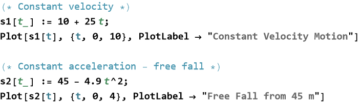
For example, a car travels at a constant 25 m/sec starting from position ![]() m. Its position at time t is x(t)=10+25t. After 8 seconds it is at x(8)=210 m.
m. Its position at time t is x(t)=10+25t. After 8 seconds it is at x(8)=210 m.
Definition 23.20 Constant Acceleration Motion: When acceleration is constant (![]() ), we can integrate step by step, first with velocity
), we can integrate step by step, first with velocity
![]()
(23.153)
and then position
![]()
(23.154)
Exercise 23.61: Verify these results. In showing them true, the definition becomes a theorem.
Let’s say that an object is dropped (![]() ) from height 45 m under gravity (a=−9.8
) from height 45 m under gravity (a=−9.8 ![]() ). Position s then
). Position s then ![]() . We can calculate the time to hit ground (s=0) is
. We can calculate the time to hit ground (s=0) is ![]() seconds.
seconds.
In another example, a car accelerates from rest at a=2 ![]() for 10 seconds. The final velocity is v(10)=0+2×10=20 m/sec. Then the distance traveled is
for 10 seconds. The final velocity is v(10)=0+2×10=20 m/sec. Then the distance traveled is ![]() m.
m.
We can visualize this kind of thing in Wolfram Language.
Exercise 23.62: Begin with Definition 23.18. Copy this into your notebook. Reflect on its meaning for a few minutes. Note any thoughts that come to mind. How would you explain this to someone sitting in front of you. Write this down. Do this for each definition and principle.
Exercise 23.63: A train moves at a constant velocity of 22 m/sec. At time t=0, it is at position ![]() meters.
meters.
1) Write the position function.
2) How far has the train traveled after 45 seconds?
3) How long does it take to reach the 2 km mark?
Exercise 23.64: A car starts from rest (![]() ) and accelerates at a constant rate of ( 3.5 )
) and accelerates at a constant rate of ( 3.5 ) ![]() .
.
1) Write the velocity and position functions.
2) How fast is the car moving after 8 seconds?
3) How far has it traveled in those 8 seconds?
4) Use the equation ![]() to verify your answer in part 3).
to verify your answer in part 3).
Exercise 23.65: A ball is thrown upward with initial velocity 15 m/sec from a height of 25 meters. Take g=−9.8 ![]() (downward).
(downward).
1) Write the velocity and position functions.
2) How long does it take to reach maximum height?
3) What is the maximum height above the ground?
4) When does the ball hit the ground?
Exercise 23.66: A particle has acceleration a(t)=4 ![]() and initial velocity
and initial velocity ![]() m/sec at t=0, starting from
m/sec at t=0, starting from ![]() m.
m.
1) Write the velocity function.
2) Write the position function.
3) At what time(s) is the particle at rest?
4) What is its position at that time?
Exercise 23.67: A truck brakes with constant acceleration a=−2.5 ![]() . It is traveling at 30 m/sec when the brakes are applied.
. It is traveling at 30 m/sec when the brakes are applied.
1) How long does it take to stop?
2) How far does it travel before stopping?
3) Use two different kinematic equations to solve part 2) and confirm the answers match.
Exercise 23.68
1) Define in Wolfram Language the position function for an object with initial position 0, initial velocity 12 m/sec, and constant acceleration -9.8 ![]() .
.
2) Use Plot to graph position vs. time from t=0 to the time it returns to the ground.
3) Use Integrate to compute total displacement from t=0 until it hits the ground.
4) How do the kinematic equations you derived using derivatives and integrals compare to the standard memorized formulas? Which approach do you find more insightful for understanding motion?
The Method of Substitution
Many integrals look complicated at first glance, but they are actually the result of a chain rule applied in reverse. If we can recognize a composite function inside the integrand, we can make a clever change of variable—called substitution—that simplifies the expression dramatically. This method turns a hard integral into a much easier one, often reducing it to a basic power, trigonometric, or exponential form we already know how to integrate.
Principle 23.9 Substitution as the Reverse of the Chain Rule: If an integrand contains a composite function whose derivative appears (or nearly appears) elsewhere, we can substitute to undo the chain rule.
Algorithm 23.1 The Method of Substitution:
Look for an “inner” function u=g(x) whose derivative g'(x) appears (or is a constant multiple of something) in the integrand.
Compute du=g'(x) dx.
Rewrite the entire integral in terms of u.
Integrate with respect to u.
Substitute back to the original variable (or evaluate definite limits if given).
Let’s say we need to evaluate ![]() . Step 1, Let u=2x+3. Step 2, so du=2 dx and dx=du/2. Final steps,
. Step 1, Let u=2x+3. Step 2, so du=2 dx and dx=du/2. Final steps,
![]()
(23.155)
For a second example, w have ∫sin (3 x) dx. Step 1, u=3 x. Step 2, du=3 dx, so dx=du/3. Final steps,
![]()
(23.156)
We can produce similar results using Wolfram Language.
![]()
![]()
Exercise 23.69: Begin with Principle 23.9. Copy this into your notebook. Reflect on its meaning for a few minutes. Note any thoughts that come to mind. How would you explain this to someone sitting in front of you. Write this down. Do this for the algorithm, too.
Exercise 23.70: Use the method of substitution to find each indefinite integral. Include the constant of integration +c.
1) ![]()
2) ![]()
3) ![]()
Exercise 23.71: Evaluate:
1) ∫sin (5x) dx
2) ∫cos (2x + 1)dx
3) ![]()
Exercise 23.72: Evaluate the following definite integrals using substitution and changing limits:
1) ![]()
2) ![]()
3) ![]()
Exercise 23.73: A particle has velocity ![]() m/sec.
m/sec.
1) Use substitution to find the general position function.
2) If s(0)=5 m, find the specific position function.
3) How far has the particle traveled from t=0 to t=2 seconds?
Work Done by a Variable Force
In earlier lessons you learned that the work done by a constant force is simply W=F Δ x (or more generally ![]() ). This works beautifully when the force never changes. But in the real world forces almost always vary with position—think of a spring whose restoring force grows linearly with stretch, gravity that weakens with distance, or the drag on a falling object. So far, this lesson has equipped you with the definite integral as a way to add up infinitely many tiny contributions. Here we apply that tool directly to the physical concept of work. You will see how the integral turns the varying force into a single total, interpret the result geometrically as an area under a curve, and connect it to the work-energy theorem you will meet formally in Lesson 38. By the end of this section you will be able to compute the work done by any force that depends on one-dimensional position and understand why integration is indispensable in theoretical physics.
). This works beautifully when the force never changes. But in the real world forces almost always vary with position—think of a spring whose restoring force grows linearly with stretch, gravity that weakens with distance, or the drag on a falling object. So far, this lesson has equipped you with the definite integral as a way to add up infinitely many tiny contributions. Here we apply that tool directly to the physical concept of work. You will see how the integral turns the varying force into a single total, interpret the result geometrically as an area under a curve, and connect it to the work-energy theorem you will meet formally in Lesson 38. By the end of this section you will be able to compute the work done by any force that depends on one-dimensional position and understand why integration is indispensable in theoretical physics.
Let us begin.
Definition 23.20 Work Done by a Variable Force: Suppose a particle moves along the x-axis from position x=a to x=b under the influence of a force F(x) that depends on position. We divide the interval [a, b] into n tiny subintervals, each of width ![]() . In the ith subinterval the force is approximately constant and equal to its value at some point
. In the ith subinterval the force is approximately constant and equal to its value at some point ![]() inside that subinterval. The tiny bit of work done in that piece is therefore
inside that subinterval. The tiny bit of work done in that piece is therefore
![]()
(23.157)
The total work is the sum of all these pieces
![]()
(23.158)
If we now let the maximum width of the subintervals approach zero (![]() ), the sum becomes the definite integral
), the sum becomes the definite integral
![]()
(23.159)
(If the force and displacement are in the same direction we drop the vector notation; otherwise we use the scalar product, but in one dimension this reduces to the scalar form above when signs are handled carefully.)
This definition is exact in the limit. It does not assume the force is constant, linear, or anything else—only that F(x) is integrable on [a, b].
The integral ![]() is precisely the signed area between the curve y=F(x) and the x-axis from a to b. Positive force (to the right) above the axis contributes positive work, while negative force contributes negative work (energy is extracted from the system).
is precisely the signed area between the curve y=F(x) and the x-axis from a to b. Positive force (to the right) above the axis contributes positive work, while negative force contributes negative work (energy is extracted from the system).
A classic case is an ideal spring. Hooke’s law tells us the restoring force is
![]()
(23.160)
where k>0 is the spring constant and x is the displacement from equilibrium (positive x stretches the spring). Suppose we slowly stretch the spring from x=0 to ![]() . The work done by the external agent is the negative of the work done by the spring itself
. The work done by the external agent is the negative of the work done by the spring itself
![]()
(23.161)
This is exactly the elastic potential energy stored in the spring. You will see this again when we discuss conservation of energy.
You can visualize and compute this instantly using the Wolfram Language.
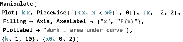
The shaded area from 0 to ![]() equals
equals ![]() .
.
Algorithm 23.2 Calculating the Work Done by a Force: To compute work done by any F(x):
Write the force as a function of position.
Determine the limits of integration (initial and final positions).
Evaluate the definite integral.
Interpret the sign: positive work means energy added to the system by the force; negative means energy removed.
Suppose ![]() (in newtons) and the particle moves from x=0 to x=3 m. Then
(in newtons) and the particle moves from x=0 to x=3 m. Then
![]()
(23.162)
As it happens, the net work done on an object equals its change in kinetic energy. For a variable force this becomes the powerful statement
(23.163)
This is why integration appears so often in mechanics, it lets us go directly from force laws to energy changes without solving the full equation of motion first.
Principles
Principle 23.10: The work done by a variable force is the limit of the sum of infinitesimal force-displacement products. This is exactly what the definite integral computes.
Principle 23.11: When force and displacement are parallel, work equals the area under the F(x) versus x curve (with sign).
Principle 23.12: The sign of the work tells us the direction of energy transfer: positive work increases the mechanical energy of the system (from the point of view of that force); negative work decreases it.
Exercise 23.74: Begin with Definition 23.20. Copy this into your notebook. Reflect on its meaning for a few minutes. Note any thoughts that come to mind. How would you explain this to someone sitting in front of you. Write this down. Do this for the algorithm, and each principle.
Exercise 23.75: Why does the integral automatically handle the varying force while the simple F Δ x formula cannot?
Exercise 23.76: A force F(x)=5x−2 N acts on a particle from x=1 m to x=3 m. Compute the work done. Sketch the force graph and shade the area.
Exercise 23.77: For the spring k=200 N/m stretched from 0 to 0.1 m, compute the work done by the spring and by the external hand. Explain the signs.
Exercise 23.78: Use Wolfram Language to define a force function, integrate it symbolically and numerically, and plot the force with the accumulated work as a running integral. Experiment with different forces (e.g., inverse-square, exponential decay).
Exercise 23.79: Think of a real physical situation (e.g., a bungee cord, variable gravity near Earth, air resistance). Write the force law and set up (but do not necessarily solve) the integral for the work.
Summary
Summarize this lesson.
For Further Study
Jerrold E. Marsden, Alan Weinstein, (1985), Calculus I. Springer-Verlag, New York. You can download it for free from CalTech: https://www.cds.caltech.edu/~marsden/volume/Calculus
Jerrold E. Marsden, Alan Weinstein, (1985), Calculus II. Springer-Verlag, New York. You can download it for free from CalTech: https://www.cds.caltech.edu/~marsden/volume/Calculus
Leonard Susskind, George Hrabovsky, (2011), The Theoretical Minimum: What You Need to Know to Start Doing Physics, Basic Books. This is the perfect next step. It teaches exactly the mathematical and conceptual toolkit (including more advanced integration applications in mechanics) that a serious amateur needs to think like a theoretical physicist. It starts from classical mechanics and builds the foundation for everything that follows in your series. Many readers use it alongside or right after self-made courses like yours.
Silvanus Thompson, (1914), Calculus Made Easy. MacMillan and Co. Released by The Project Gutenberg in 2012. This book has inspired generations of physicists and engineers precisely because it removes fear and reveals beauty—exactly what you’re doing in your course. Many people who later tackle The Theoretical Minimum started with Thompson and say it gave them the courage to continue.
3Blue1Brown – “Integration and the Fundamental Theorem of Calculus” (Chapter 8, Essence of Calculus)
Grant Sanderson’s visually stunning animations make the why behind integrals unforgettable — turning tiny accumulations into total work, area, and the fundamental theorem. This directly supports your “Work Done by a Variable Force” section.
Watch here: https://www.youtube.com/watch?v=rfG8ce4nNh0
Professor Leonard – Calculus 1 Lecture 4.1: An Introduction to the Indefinite Integral
Thorough, blackboard-style lectures from a patient teacher. Perfect for serious amateurs who want every detail explained slowly and clearly, including integration by parts.
Watch here: https://www.youtube.com/watch?v=b2ZFpE_yrLg
Full Calculus 1 playlist: https://www.youtube.com/playlist?list=PLF797E961509B4EB5