Lesson 22 Calculus 3 Applications of Derivatives

“The real purpose of calculus is to understand change — not just to compute it, but to feel it in your bones.”—Richard Feynman
“To those who do not know mathematics, it is difficult to get across a real feeling as to the beauty, the deepest beauty, of nature… if you want to learn about nature, it is necessary to understand the language that she speaks in.”—Richard Feynman

Introduction

We have learned what a derivative is and how to compute it. But knowing the derivative is only the beginning. The real power of calculus emerges when we use derivatives to understand the behavior of the physical world—to find maximums and minimums, to analyze motion, to relate different rates of change, and to approximate complicated functions with simple ones. The derivative is not merely a slope on a graph. It is a tool that reveals how things change, how systems optimize themselves, how forces and energies interact, and how we can predict the future behavior of physical systems from their present state. In this lesson we move from pure computation to genuine application. We will use derivatives to solve real problems in mechanics, electricity, optimization, and motion. You will see how the abstract idea of an instantaneous rate of change becomes one of the most practical and powerful tools in all of theoretical physics.

As we work through these topics, you will begin to see the world differently. Every curve, every motion, every optimization problem will invite you to ask, “What is the derivative telling me here?” This is where calculus stops being a collection of rules and starts becoming a way of thinking—a language for describing change itself.

You have already built a strong foundation. Now it is time to put that foundation to work and discover how derivatives illuminate the inner workings of nature.

Let us begin.

The Tangent Line

Imagine zooming in closer and closer on a smooth curve at a particular point. No matter how much you magnify it, the curve begins to look more and more like a straight line. That straight line which best matches the curve right at that point—touching it and sharing the same direction—is one of the most important ideas in calculus.

This line is called the tangent line. The tangent line at a point on a curve is the unique straight line that passes through the point and has the same instantaneous rate of change (slope) as the curve at that exact location. It is the best linear approximation to the curve near that point.

Definition 22.1 Equation of the Tangent Line: If a function f(x) is differentiable at x=a, then the equation of the tangent line at the point (a,f(a)) is

(22.1)

Here f'(a) is the slope of the curve at x=a, and the expression f(a)+f'(a)(x-a) is the linear approximation to f(x) near x=a.

Say we want to find the tangent line to at x=3. We can write f(3)=9, and f'(x)=2x, so f'(3)=6.

We then write (22.1), y=9+6(x-3=9+6x-18=6x-9, so the tangent line is y=6x-9.

The position of a particle moving along a line is given by   meters, where t is in seconds. At t=2 seconds s(2)=2 m  and the velocity is ,  so s'(2)=3 m/s,

Then the tangent line to the position-time graph at t=2 is s(t)≈2+3(t−2). This line gives the best linear approximation to the particle’s position near t=2 seconds. Its slope is exactly the instantaneous velocity.

We can see the plots.

You can clearly see how the tangent line touches the parabola at x=3 and matches its slope perfectly.

The tangent line is your first powerful application of the derivative. It turns the abstract concept of “instantaneous rate of change” into a concrete, usable straight line that helps us understand and predict the local behavior of functions — a skill you will use again and again in physics.

Principles

Principle 22.1 Tangent Line as the Best Local Approximation: Near a point where a function is differentiable, the tangent line gives the most accurate straight-line approximation to the curve. The closer x is to the point of tangency, the better the approximation.

Principle 22.2 Geometric Interpretation of the Derivative: The derivative f'(a) is geometrically the slope of the tangent line to the curve at x=a. This is the fundamental link between the algebraic definition of the derivative and its geometric meaning.

Theorems

Theorem 22.1 Existence of the Tangent Line: If a function f is differentiable at x=a, then the tangent line to the graph of f exists at the point (a, f(a)).

Proof of Theorem 22.1: This is a direct proof. By the definition of differentiability at x=a, the following limit exists and is a finite number

(22.2)

where m=f'(a) is the derivative at x=a. This limit means that as x approaches a, the slope of the secant line connecting the points (a, f(a)) and (x, f(x)) gets arbitrarily close to the value m. Consider the straight line passing through the point (a, f(a)) with slope m. Its equation is

(22.3)

We claim that this line is the tangent line to the graph of f at x=a. To justify this, note that the difference between the function value f(x) and the value predicted by this line is

(22.4)

Because , the term in parentheses approaches 0 as x→a. Therefore,

(22.5)

This shows that the straight line y=f(a)+m(x−a) approximates f(x) with an error that goes to zero faster than ∣x−a∣ as x approaches a. In other words, this line is the unique straight line that best matches the curve at the point (a, f(a)), both in position and in slope.

Thus, the tangent line exists and is given by y=f(a)+f'(a)(x−a). QED

Theorem 22.2 Tangent Line Approximation Error: For a differentiable function, the error in the linear approximation ∣f(x)−L(x)∣ approaches zero faster than ∣x−a∣ as x→a

Proof of Theorem 22.2: This is a direct proof that requires us to construct an error term that satisfies a limit condition. By the definition of differentiability at x=a, we have

(22.6)

This means that for every ε>0, there exists a δ>0 such that if 0<∣x−a∣<δ, then

(22.7)

Now consider the error ∣f(x)−L(x)∣

(22.8)

Taking absolute values

(22.9)

Therefore

(22.10)

From the definition of the derivative, as x→a

(22.11)

So the error is the product of two things going to zero, ∣x−a∣ and another small quantity. That makes the error shrinks faster than ∣x−a∣. QED

Exercise 22.1: Begin with Definition 22.1. Copy this into your notebook. Reflect on its meaning for a few minutes. Note any thoughts that come to mind. How would you explain this to someone sitting in front of you. Write this down. Do this for each principle, theorem, and proof.

Exercise 22.2: Find the equation of the tangent line to the curve at x=2.
    1) Compute f(2) and f'(2).


    2) Write the equation of the tangent line.
    3) Draw the curve and the tangent line.

Exercise 22.3: The position of a particle along a straight line is given by meters, where t is in seconds.
    1) Find the equation of the tangent line to the position-time graph at t=1 second.


    2) What physical quantity does the slope of this tangent line represent?
    3) Use the tangent line to estimate the position at t=1.2 seconds.

Exercise 22.4: Consider at x=4.
    1) Find the equation of the tangent line at this point.


    2) Use the tangent line to approximate and .
    3) Compare your approximations with the actual values.

Exercise 22.5: Define f(x)=sin x in the Wolfram Language.
    1) Find the tangent line to f(x) ay x=π/3.


    2) Plot both f(x) and its tangent line on the same graph.
    3) Use Manipulate to explore the tangent line at different points and observe how well it approximates the sine curve near the point of tangency.

Exercise 22.6: For the function :
    1) Find the points where the tangent line is horizontal.


    2) Write the equations of the tangent lines at those points.
    3) Sketch the graph and all horizontal tangent lines.

Exercise 22.7:
    1) Explain in your own words what the tangent line represents both geometrically and physically.


    2) When is the tangent line a good approximation to the curve, and when does it become a poor approximation?
    3) Give one real-world situation (from physics or engineering) where the tangent line approximation is very useful, and explain why.

The Normal Line

We have seen how the tangent line matches the direction of a curve at a given point. Now we ask, “What is the line that runs perpendicular to the tangent line at that same point?” This line is called the normal line. The normal line at a point on a curve is the unique straight line that passes through the point and is perpendicular to the tangent line there. While the tangent line tells us the direction of motion or slope, the normal line points in the direction “straight out” from the curve—a direction that appears frequently in physics when we talk about forces pushing or pulling perpendicular to a surface.

If the tangent line at x=a has slope m=f'(a), then the normal line has slope

(22.12)

Definition 22.2 The Equation of the Normal Line : At the point (a, f(a)) this equation is

(22.13)

Let’s say we want to find the normal line to at x=2. We have f(2)=4 and f'(x)=2x, so f'(2)=4. Then the slope of the normal line at the point is 1/4.

Then the equation of normal line is

(22.14)

Next we suppose a particle is sliding on the curve . At the point where x=1, the tangent slope is f'(1)=1. The normal line has slope −1. The direction of the normal line tells us the direction of the normal force that the surface exerts on the particle—perpendicular to the surface at the point of contact. This is essential in problems involving friction, inclined surfaces, and constrained motion.

We can see what this sort of thing looks like using Wolfram Language.

You can clearly see that the normal line is perpendicular to the tangent line at the point of contact.

The normal line completes the picture started by the tangent line. Together, they give us the two fundamental directions at any point on a curve — along the path and perpendicular to it. This pair of directions will prove essential when we study forces, motion on curves, and optimization in the sections ahead.

Definitions

Definition 22.3: Two lines are perpendicular if the product of their slopes is −1 (provided neither is vertical). This is the algebraic condition that guarantees a right angle between them.

Definition 22.4: The normal direction at a point on a curve is the direction perpendicular to the tangent vector at that point. It points “outward” from the local curvature of the path.

Definition 22.5: A constraint force is a force (such as the normal force) whose direction is determined by the geometry of the surface or path, acting to keep an object on that path.

Principles

Principle 22.3: The normal line provides the natural direction for any force that prevents an object from penetrating or leaving a surface (the normal force in mechanics).

Principle 22.4: In constrained motion along a curve, forces can be decomposed into tangential components (which change speed) and normal components (which change direction). The normal line defines the direction of the normal component.

Principle 22.5 (Slope Relationship): If a line has slope m, then any line perpendicular to it has slope −1/m (the negative reciprocal).

Theorems

Theorem 22.3: At any point where a curve is differentiable, there exists a unique normal line (perpendicular to the tangent line) passing through that point.

Proof of Theorem 22.3: This is a direct proof by cases. Since f is differentiable at x=a, the derivative f'(a) exists and is a real number. This means the tangent line at x=a exists and has a well-defined slope m=f'(a). We consider two cases.

Case 1: f'(a)≠0 (the tangent line is non-vertical)

The slope of any line perpendicular to the tangent line must be the negative reciprocal

(22.15)

By the point-slope form of the equation of a line, there is exactly one line that passes through the point (a, f(a)) with slope

(22.16)

Thus, a unique normal line exists in this case.

Case 2: f'(a)=0 (the tangent line is horizontal)

A horizontal line has slope 0. Any line perpendicular to a horizontal line must be vertical. The unique vertical line passing through (a, f(a)) is x=a. This is the normal line in this case.

In both cases, the normal line exists and is unique. Therefore, at every point where the curve is differentiable, there is a unique normal line perpendicular to the tangent line passing through that point. QED

Theorem 22.4 (Perpendicularity Test): Two lines with slopes and are perpendicular if and only if .

Proof of Theorem 22.4: This is a direct proof. We prove both sides of the argument.

First side: Suppose the two lines are perpendicular.

Let have slope and have slope . Since the lines are perpendicular, they form a right angle (90°) at their intersection point.

Consider the right triangle formed by the two lines and the horizontal axis. The angle that makes with the positive x-axis satisfies

(22.17)

Similarly, the angle that makes with the positive x-axis satisfies

(22.18)

Because the lines are perpendicular, the difference in their angles is 90°

(22.19)

Taking the tangent of both sides and using the tangent subtraction formula

(22.20)

and this is is undefined! For the tangent to be undefined, the denominator must be zero

(22.21)

We now consider the other direction: Suppose .Then (assuming ). This means is the negative reciprocal of . By the converse of the argument above, the angle between the lines must be 90°, so the lines are perpendicular.

There are two special cases:

If one line is horizontal =0), then for to hold, would need to be undefined (a vertical line). A horizontal line and a vertical line are indeed perpendicular.

Vertical lines (undefined slope) are perpendicular only to horizontal lines.

Thus, the theorem holds in all cases. QED

Exercise 22.8: Begin with Definition 22.2. Copy this into your notebook. Reflect on its meaning for a few minutes. Note any thoughts that come to mind. How would you explain this to someone sitting in front of you. Write this down. Do this for each definition, principle, theorem, and proof.

Exercise 22.9: Find the equation of the normal line to the curve at x=2.
    1) Compute f(2) and f'(2).


    2) Determine the slope of the normal line.
    3) Write the full equation of the normal line.

Exercise 22.10: A particle is constrained to move along the parabolic path . At the point (2, 1):
    1) Find the equation of the normal line.


    2) In which direction does the normal line point relative to the curve?
    3) Explain physically what this normal direction represents for a bead sliding on a wire shaped like this parabola.

Exercise 22.11: Consider f(x)=sin⁡ x at x=π/4.
    1) Find the equations of both the tangent line and the normal line at this point.


    2) Verify that the two lines are perpendicular by showing that the product of their slopes is −1.
    3) Plot both lines along with the sine curve using Wolfram Language.

Exercise 22.12: Define in Wolfram Language.
    1) Find the normal line at x=1.


    2) Plot the curve, the tangent line, and the normal line together on the same graph.
    3) Use Manipulate to explore the normal line at different points on the curve.

Exercise 22.13: A car is traveling along a road shaped like (in meters). At the point where x=10 m:
    1) Find the slope of the normal line.


    2) Describe the direction in which the road exerts a normal force on the car’s tires at that point.
    3) Why is this normal direction important for the car’s stability on the curved road?

Exercise 22.14:
    1) Explain in your own words the geometric relationship between the tangent line and the normal line.


    2) Why is the normal line particularly important in physics when analyzing forces on curved surfaces or paths?
    3) Give one real-world example (other than a particle on a wire) where the direction of the normal line plays a critical role.

The Direction of Force

We have seen that the tangent line at a point on a curve gives the instantaneous direction in which an object is moving. This simple geometric idea has profound consequences when we think about forces acting on that object. Here, at any moment, a force can act either along the direction of motion (parallel to the tangent) or perpendicular to the direction of motion. Forces parallel to the tangent change the object’s speed. Forces perpendicular to the tangent change the object’s direction without directly changing its speed at that instant. This distinction—tangential versus perpendicular components of force—is one of the most useful ways to analyze motion along curved paths.

A force acting in the direction of the tangent (or opposite to it) affects how fast the object is moving. It is responsible for tangential acceleration. If the tangential force is in the same direction as velocity then the object speeds up. If the tangential force is opposite to velocity then the object slows down.

A car is driving over a parabolic hill has its velocity always tangent to the road. The component of gravity along the tangent direction either helps accelerate the car downhill or slows it uphill. This tangential component directly changes the car’s speed.

At any point in a pendulum’s swing, the velocity is tangent to the circular arc. The component of gravity along the tangent direction slows the bob as it rises and speeds it up as it falls. This tangential force determines the change in speed.

A force acting perpendicular to the tangent changes the direction of motion—it pulls the object sideways, keeping it on a curved path. This perpendicular force is what prevents an object from flying off in a straight line when moving along a curve (think of a car turning a corner or a satellite orbiting Earth).

We can visualize this.

This way of thinking—separating forces into tangential and perpendicular components—will become increasingly powerful as we continue through this lesson. It is the foundation for understanding circular motion, constrained paths, and many other important physical situations.

Definitions

Definition 22.6 Tangential Force: A force is tangential at a point on a curve if it acts parallel (or anti-parallel) to the tangent line at that point. A tangential force changes the speed (magnitude of velocity) of the object.

Definition 22.7 Perpendicular (Normal) Force: A force is perpendicular (or normal) at a point on a curve if it acts at a right angle to the tangent line at that point. A perpendicular force changes the direction of motion without directly changing the speed at that instant.

Definition 22.8 Tangential Acceleration: The component of acceleration along the tangent direction, responsible for changing the object’s speed

(22.22)

where v is the speed.

Principles

Principle 22.6 Force Direction Principle: At any point on a curved path, any net force can be decomposed into two mutually perpendicular components. A tangential component (parallel to velocity) that changes the object’s speed. A perpendicular (normal) component that changes the object’s direction.

Theorems

Theorem 22.5 Decomposition of Force: Any force acting on an object moving along a curve can be uniquely written as where is parallel to the tangent and is parallel to the normal.

Proof of Theorem 22.5: This is a direct proof based on the vector materials introduced in Lesson 16. At any point on a smooth curve, we have two well-defined perpendicular directions, the tangent direction, given by the tangential vector (or any nonzero multiple of it), and the normal direction, given by the normal vector , and that is perpendicular to .

Step 1: Existence of the Decomposition

Since and are perpendicular and nonzero, they form a basis for the two-dimensional plane containing the force . Therefore, there exist unique scalars and such that

(22.23)

where and are the unit tangent and unit normal vectors, respectively. We then define

(22.24)

and

(22.25)

This gives the required decomposition .

Step 2: Uniqueness

Suppose there is another decomposition , where is parallel to the tangent and is parallel to the normal.

Then

(22.26)

The left side is parallel to the tangent, while the right side is parallel to the normal. The only vector that is parallel to both the tangent and the normal is the zero vector (because the tangent and normal are perpendicular). Therefore,

(22.27)

this implies and . The decomposition is unique. QED

Exercise 22.15: Begin with Definition 22.6. Copy this into your notebook. Reflect on its meaning for a few minutes. Note any thoughts that come to mind. How would you explain this to someone sitting in front of you. Write this down. Do this for each definition, principle, theorem, and proof.

Exercise 22.16: A particle moves along the curve . At the point (1,−2), the derivative is f'(1)=0.
    1) What is the direction of the tangent line at this point?


    2) If a force acts vertically upward at this point, is it tangential or perpendicular to the direction of motion?
    3) Would this force change the particle’s speed or its direction?

Exercise 22.17: A car is driving over a hill shaped like (in meters). At the point where x=10  m, the slope of the road is f'(10)=2.


    1) Find the angle the tangent makes with the horizontal.


    2) If the car’s weight has a component parallel to the tangent, explain whether this component increases or decreases the car’s speed as it goes over the hill.
    3)  Sketch the situation showing the tangent direction and the tangential force component.

Exercise 22.18: A simple pendulum swings along a circular arc.


    1) At the lowest point of the swing, in which direction is the velocity (tangent direction)?


    2) At that same point, is the tension in the string tangential or perpendicular to the motion?
    3) Which force component (gravity or tension) is responsible for changing the bob’s speed near the bottom? Explain.

Exercise 22.19: Consider the curve at x=1.


    1) Plot the curve, the tangent line, and an arrow showing the tangent direction (velocity).


    2) Add a second arrow showing a perpendicular direction.
    3) Use Manipulate to move the point along the curve and observe how the tangent direction changes.

Exercise 22.20: A roller coaster car moves along a curved track.


    1) At the top of a hill, explain whether the net force along the tangent direction is likely speeding the car up or slowing it down.


    2) At the bottom of a valley, is the tangential force component increasing or decreasing the speed?
    3) Why must engineers carefully design the perpendicular forces (normal forces) at high-speed curves?

Exercise 22.21:


    1) Explain in your own words the difference between a tangential force and a perpendicular force on a curved path.


    2) Give two real-world examples (not from the section) where tangential forces are dominant and two where perpendicular forces are dominant.
    3) Why is being able to separate forces into tangential and perpendicular components such a powerful tool in theoretical physics?

The Normal Force

When an object rests on a surface or moves along a curved path, the surface pushes back on the object. This push is always perpendicular to the surface at the point of contact. It prevents the object from sinking into the surface or flying off it.

This perpendicular push is called the normal force. (recall that we introduced this type of force in Lesson 15). The normal force is the force exerted by a surface on an object that is in contact with it, directed perpendicular (normal) to the surface at the point of contact. It arises precisely to counteract any tendency of the object to penetrate the surface. Its direction is given by the normal line we studied earlier.

The normal force is always perpendicular to the surface. It is a contact force—it exists only when two objects are touching. Its magnitude adjusts automatically to prevent penetration (it is a “constraint force”). It does not do work when the object slides along the surface, because it is perpendicular to the direction of motion (the tangent direction).

For example a 5 kg block rests on a flat table. The normal force exactly balances the weight of the block,

(22.28)

The normal line here is vertical—straight up, perpendicular to the table.

For another example, a block sits on a ramp inclined at 30°. The normal force is perpendicular to the ramp surface

(22.29)

This force prevents the block from sinking into the ramp. The component of gravity parallel to the ramp (tangential) causes the block to slide down.

Yet another example is when a car drives over a parabolic hill . At the top of the hill, the normal force points along the normal line (downward toward the center of curvature). At high speeds, the required centripetal force may exceed what gravity can provide, and the normal force can drop to zero—the car loses contact with the road.

We can see what this looks like in Wolfram Language.

The normal force is one of the most common yet subtle forces in mechanics. Learning to recognize its direction—always along the normal line—is a crucial skill that will help you analyze constrained motion, circular paths, inclined planes, and many other important physical systems in the sections ahead.

Principles

Principle 22.7 Direction of the Normal Force: The normal force is always perpendicular to the surface at the point of contact. Its direction is given by the normal line to the curve or plane at that point.

Principle 22.8 Nonworking Nature of the Normal Force: When an object slides along a surface, the normal force does no work because it is perpendicular to the instantaneous direction of motion (the tangent direction). Thus, .

Principle 22.9 Automatic Adjustment: The magnitude of the normal force automatically adjusts to whatever value is necessary to prevent the object from sinking into or flying off the surface (within the limits of the material’s strength).

Principle 22.10 Free-Body Diagram Rule: In any free-body diagram (a concept we introduced in the section Using Arrows to Represent Quantities in Lesson 16, the normal force is drawn perpendicular to the surface, pointing away from the surface toward the object.

Exercise 22.22: Begin with Principle 22.76. Copy this into your notebook. Reflect on its meaning for a few minutes. Note any thoughts that come to mind. How would you explain this to someone sitting in front of you. Write this down. Do this for each principle.

Exercise 22.23: A 12 kg box rests on a horizontal floor.


    1) Draw a free-body diagram (from Lesson 16) and calculate the magnitude of the normal force.


    2) In which direction does the normal force act relative to the surface?
    3) What would happen if the normal force were suddenly smaller than the weight of the box?

Exercise 22.24: A 8 kg block is placed on a frictionless ramp inclined at 35° to the horizontal.


    1) Find the magnitude of the normal force acting on the block.


    2) Explain why the normal force is not equal to the full weight ( mg ).
    3) Draw the free-body diagram showing the normal force perpendicular to the ramp.

Exercise 22.25: A car of mass 1200 kg drives over the top of a parabolic hill described by (in meters). At the crest (x=0), the car is traveling at 25 m/sec.


    1) At the top, in which direction does the normal force point?


    2) If the normal force becomes zero, what is the maximum speed the car can have without losing contact with the road? (Use g=9.8  ).
    3) Explain the role of the normal force in keeping the car on the curved path.

Exercise 22.26: Consider the curve .


    1) At x=10, calculate the slope of the tangent and the slope of the normal line.


    2) Plot the curve, the tangent line, and the normal line at this point.
    3) Add an arrow showing the direction of the normal force on an object at that point.

Exercise 22.27: A person of mass 70 kg stands in an elevator.


    1) When the elevator accelerates upward at 2 , what is the normal force (apparent weight) exerted by the floor?


    2) When the elevator accelerates downward at 3 , what is the normal force?
    3) Explain why the normal force changes even though the person’s actual weight is constant.

Exercise 22.28:


    1) Explain in your own words why the normal force is always perpendicular to the surface.


    2) Give two situations where the normal force is equal to the weight and two situations where it is not.
    3) Why is it important in physics to distinguish between the normal force (perpendicular) and frictional or tangential forces (parallel to the surface)?

Linear and Angular Kinematics

We have already seen how the derivative describes instantaneous rates of change. Now we apply that idea to two closely related types of motion. Motion along a straight line and motion around a circle or axis. Linear kinematics describes motion along a straight path using position, velocity, and acceleration. Angular kinematics does the same for rotational motion using angular position, angular velocity, and angular acceleration. The mathematics is strikingly similar—derivatives connect them both.

Definition 22.9 Linear Kinematics: For an object moving along a straight line with position s(t). The time rate of change of the position function (the time derivative) is what we call the velocity

(22.30)

The time rate of change of the velocity (the time derivative) is what we call the acceleration

(22.31)

Definition 22.10 Angular Kinematics: For an object rotating about a fixed axis with angular position θ(t) (in this case measured in radians). The time derivative of the angular position is the angular velocity

(22.32)

The time derivative of the angular velocity is the angular acceleration

(22.33)

For circular motion of radius r, linear and angular quantities are related by

(22.34)

We can think of this as unrolling the circle to treat it as one-dimensional motion.

We can split acceleration in tangential acceleration

(22.35)

and centripetal (radial) acceleration

(22.36)

These relationships show that rotational motion can be analyzed using the same derivative tools we use for linear motion.

For example a particle moves along a line with position meters. The velocity is . Then the acceleration is a(t)=18t−12.

At t=1 sec we get v(1)=9-12+4=1 m/sec, and a(1)=18-12=6 , this is is speed up.

Another example has a wheel that rotates with angular position radians. The angular velocity is . The angular acceleration is α(t)=12t−10.

At t=2 sec we have angular velocity ω(2)=4 . If the wheel has radius 0.5 m, the linear (tangential) speed at that instant is v=r ω=0.5×4=2 m/sec.

We can see what this looks like in Wolfram Language.

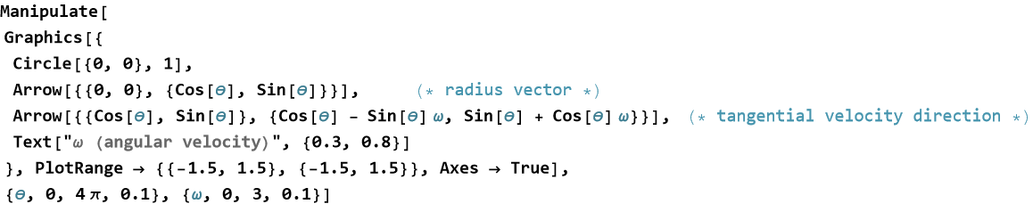
Linear and angular kinematics are two sides of the same coin. Mastering both—and the connections between them—gives you powerful tools for analyzing almost any kind of motion you will encounter in theoretical physics.

Exercise 22.28: Begin with Definition 22.9. Copy this into your notebook. Reflect on its meaning for a few minutes. Note any thoughts that come to mind. How would you explain this to someone sitting in front of you. Write this down. Do this for each defintion.

Exercise 22.29: The position of a particle moving along a straight line is given by meters, where t is in seconds.


    1) Find the velocity function v(t) and acceleration function a(t).


    2) Determine the velocity and acceleration at t=2 seconds.
    3) Is the particle speeding up or slowing down at that instant? Explain.

Exercise 22.30: We determine that a car is accelerating at a rate of 10 miles per hour per minute.


    1) Is this a valid unit of acceleration?


    2) If we start at 5 miles per hour, how fast are we going after two minutes?

Exercise 22.31: A wheel rotates with angular position radians.


    1) Find the angular velocity ω(t) and angular acceleration α(t).


    2) Evaluate ω(1) and α(1).
    3) At t=1 sec, is the wheel speeding up or slowing down rotationally?

Exercise 22.32: A car tire has radius r=0.32 m and rotates with angular velocity rad/sec.


    1) Find the linear (tangential) speed of a point on the rim.


    2) Calculate the linear speed at t=2 seconds.
    3) Find the centripetal acceleration of a point on the rim at that time.

Exercise 22.33: A pendulum bob swings with angular position θ(t)=0.3sin⁡(4t) radians.


    1) Find the angular velocity ω(t).


    2) If the pendulum length is 1.2 m, find the linear speed of the bob as a function of time.

Exercise 22.34: Consider a wheel of radius 0.4 m with angular position radians.


    1) Define the linear position of a point on the rim (using x=r cos⁡ θ, y=r sin ⁡θ).


    2) Plot both the angular position θ(t) and the linear tangential speed v(t) from t=0 to t = 5.
    3) Use Manipulate to explore how changing the radius affects the linear quantities.

Exercise 22.35:


    1) Explain in your own words the relationship between linear velocity v and angular velocity ω.


    2) Why is it useful to describe the same motion using both linear and angular kinematics?
    3) Give one real-world example (e.g., a car wheel, a Ferris wheel, or a spinning hard drive) where both descriptions are valuable. When would you prefer angular quantities over linear ones?

Stationary Points

When we look at the graph of a function that describes a system—whether it is position, potential energy, or some other (even mathematical) quantity—certain special points often stand out. These are places where the graph flattens out momentarily, where the slope becomes zero. A stationary point is a point on the graph of a function where the derivative (the instantaneous rate of change) is exactly zero. At these points, the function is neither increasing nor decreasing for an instant—it is “stationary.” These points are incredibly important in physics because they often correspond to equilibrium positions, maximum or minimum energy states, turning points in motion, or optimal values.

Definition 22.11 Stationary Points: A point x=c where

(22.37)

is called a stationary point f(x). These are also called critical points. A critical point can also occur if the derivative does not exist at a point.

We have seen that the first derivative tells us whether a function is increasing or decreasing. The second derivative goes one level deeper—it tells us how the function is increasing or decreasing, that is, whether the graph is curving upward or downward. The concavity of a function describes the way the graph bends—whether it opens upward (like a cup) or downward (like a hill) near a point.

Definition 22.12 Concavity of a Function: Let f(x) be a twice-differentiable function. The function is concave up (or convex) on an interval if its graph lies above its tangent lines on that interval. This occurs when f''(x)>0. The function is concave down (or concave) on an interval if its graph lies below its tangent lines on that interval. This occurs when f''(x)<0. A point where the concavity changes (from up to down or down to up) is called an inflection point. At an inflection point, f''(x)=0 (and the second derivative changes sign).

Stationary points are classified into three main types:

Local Maximum: The function reaches a highest point in a small neighborhood (slope changes from positive to negative), it is concave.

Local Minimum: The function reaches a lowest point in a small neighborhood (slope changes from negative to positive), it is convex.

Point of Inflection (or Saddle Point): The slope is zero but the function does not change from increasing to decreasing (or vice versa)—the concavity changes.

These concepts lead to a set of definitions.

Definition 22.13 Local Maximum: A function f has a local maximum at x=c if there exists some open interval (c−δ,c+δ) such that f(x)≤f(c) for all x in (c−δ,c+δ). The value f(c) is called a local maximum value.

Definition 22.14 Local Minimum: A function f has a local minimum at x=c if there exists some open interval (c−δ,c+δ) such that f(x)≥f(c) for all x in (c−δ,c+δ). The value f(c) is called a local minimum value.

Definition 22.15 Extreme Point (or Extremum): A point x=c is called an extreme point (or extremum) of f if it is either a local maximum or a local minimum.

Now, is there another type of extremum, other than local? Yes,

Definition 22.16 Global (Absolute) Extrema: The value f(c) is a global maximum (absolute maximum) on an interval if f(x)≤f(c) for all x in the interval f(c) is a global minimum (absolute minimum) on an interval if f(x)≥f(c) for all x in the interval.

To locate stationary points:

Compute the first derivative f'(x).

Solve the equation f'(x)=0.

(Optional but useful) Use the second derivative test or first derivative test to classify each point (we will discuss these in a moment).

Theorem 22.6 The First Derivative Test: Let f be a function that is continuous at a point c and differentiable on an open interval containing c, except possibly at c itself. Suppose f'(c)=0 (that is, x=c). Then:

If f'(x) changes from positive to negative as x passes through c , then f has a local maximum at x=c.

If f'(x) changes from negative to positive as x passes through c, then f has a local minimum at x=c.

If f'(x) does not change sign as x passes through c, then f(c) is neither a local maximum nor a local minimum (it may be a horizontal point of inflection).

Proof of Theorem 22.6: This is a direct proof. We prove only the local maximum case (the local minimum case is symmetric, and the third case follows similarly). Assume f'(x)>0 on (c−δ,c) and f'(x)<0 on (c,c+δ), for some δ>0.

Case 1: Points to the left of c (i.e., x∈(c−δ,c))

Since f'(x)>0 on this interval, f is increasing on (c−δ,c). Therefore, for any x with c−δ<x<c, f(x)<f(c).

Case 2: Points to the right of c (i.e., x∈(c,c+δ))

Since f'(x)<0 on this interval, f is decreasing on (c,c+δ). Therefore, for any x with c<x<c+δ, f(c)>f(x).

Combining both parts: In the neighborhood (c−δ,c+δ), we have f(x)≤f(c) for all x≠c, with equality only at x=c. This is exactly the definition of a local maximum at x=c. QED

Exercise 22.36: Prove Theorem 22.1 for a local minimum.

Exercise 22.37: Prove Theorem 22.1 for a point that is neither a local maximum nor a local minimum.

Let’s say that we want to find the stationary points of .We find that

(22.38)

Exercise 22.38: Verify and explain each step in (22.15)

We now set the derivative equal to zero and solve for x

(22.39)

Let’s examine points around x=3. f'(2)=-12, f'(4)=15, so the derivative is changing from negative to positive, thus we have a local minimum.

We now examine points around x=-1, f'(-2.5)=3×-5.5×-1.5=24.75, f'(-0.5)=3×-4.5×0.5=-6.75, so the derivative is changing from positive to negative, thus we have a local minimum.

Say that we find the potential energy of a particle is given by . We can consider the derivative of the potential energy to be the force. Stationary points occur where the force equals 0, which is exactly where U'(x)=0. These points correspond to positions of equilibrium.

We can see this sort of thing in Wolfram Language.

Theorem 22.7 The Second Derivative Test: Let f be a function such that f'(c)=0 (so x=c is a stationary point) and f'' exists and is continuous in an open interval containing c.

Then:

If f'' (c) > 0, then f has a local minimum at x = c.

If f'' (c) < 0, then f has a local maximum at x = c.

If f''(c) = 0, the test is inconclusive (the point could be a local maximum, local minimum, or neither).

Proof of Theorem 22.7: This is a direct proof. We prove only the local maximum case (the local minimum case is symmetric, and the third case follows similarly). Assume f'(x)>0 on (c−δ,c) and f'(x)<0 on (c,c+δ), for some δ>0.

Case 1: Points to the left of c (i.e., x∈(c−δ,c))

Since f'(x)>0 on this interval, f is increasing on (c−δ,c). Therefore, for any x with c−δ<x<c, f(x)<f(c).

Case 2: Points to the right of c (i.e., x∈(c,c+δ))

Since f'(x)<0 on this interval, f is decreasing on (c,c+δ). Therefore, for any x with c<x<c+δ, f(c)>f(x).

Combining both parts, we see that in the neighborhood (c−δ,c+δ), we have f(x)≤f(c) for all x≠c, with equality only at x=c. This is exactly the definition of a local maximum at x=c. QED

Exercise 22.39: Prove Theorem 22.2 for a local minimum.

Exercise 22.40: Prove Theorem 22.2 for an inconclusive case.

Let’s say that . We then find the stationary points . We apply the second derivative to get, f''(x)=6x. At x=1, f''(1)=6>0⇒ a local minimum. At x=−1,  f''(−1)=−6<0⇒ a local maximum.

As another example, the potential energy of a system is . We can find and classify the equilibrium points using the Second Derivative Test. and . When we set U'(x)=0⇒x={-2,0,2}.  At x=-2 then U(-2)=32, a local minimum. At x=0 then U(0)=-16, a local maximum. At x=2 then U(2)=32, another local minimum.

Exercise 22.41: Verify these results.

For , we have f'(0)=0 and f''(0)=0. The Second Derivative Test gives no information. (We need the First Derivative Test, which shows it is a local minimum.)

Stationary points are where the derivative—the rate of change—tells us the system is momentarily balanced. Learning to find and interpret them is a fundamental skill that connects calculus directly to the concepts of equilibrium, optimization, and stability in theoretical physics.

Exercise 22.42: Begin with Definition 22.11 and copy it into your notebook. Reflect on its meaning for a few minutes. Note any thoughts that come to mind. How would you explain this to someone sitting in front of you. Write this down. Do this for each definition, theorem, and proof.

Exercise 22.43: Find all stationary points of the function .


    1) Compute the first derivative.


    2) Find the stationary points.
    3) Classify the stationary points.

Optimization

We have learned how to find stationary points using derivatives and how to classify them using the First and Second Derivative Tests. Now we turn to one of the most practical and powerful applications of calculus where we use these tools to find the best possible value of a quantity. Many real-world problems ask us to maximize or minimize something—profit, time, material used, energy, height, range, etc. When a quantity can be expressed as a function of one variable, we can use the derivative to find the optimal value by locating the highest or lowest points on the graph. This process is called optimization. We first considered this topic back in Lesson 9.

Algorithm 22.1 The General Method of Optimization: To optimize a function f(x) on a closed interval [a, b]:

Find all critical points in the open interval (a, b) by solving f'(x)=0.

Evaluate f(x) at all critical points and at the endpoints x=a and x=b.

Compare these values.

The largest is the global maximum; the smallest is the global minimum.

If the domain is not closed, we must also check behavior as x→±∞.

For example, a farmer wants to build a rectangular pen using 100 meters of fencing against a straight river (so only three sides need fencing). What dimensions give the maximum area? Let x be the width perpendicular to the river. Then the length parallel to the river is 100−2x. This gives an area of . Then A'(x)=100−4x=0⇒x=25. Then at x=25, A=1250   (maximum). The optimal pen is 25 m wide and 50 m long.

We can see a plot of this in Wolfram Language.

Optimization is one of the most satisfying applications of calculus. It shows how the derivative—the mathematics of change—can be used to find the very best outcome in a wide variety of physical, engineering, and economic situations. You will return to these ideas again and again in theoretical physics.

Definition

Definition 22.11 Optimization: The process of finding the maximum or minimum value of a function (called the objective function) subject to any given constraints on its domain.

Principles

Principle 22.17 The Endpoint Principle: When optimizing a continuous function on a closed, bounded interval [a, b], the global maximum and global minimum must occur either at a critical point in the open interval (a, b) or at one of the endpoints x=a or x=b.

Principle 22.18 First Derivative Test for Optimization: At a critical point c, if the first derivative changes from positive to negative, then f(c) is a local (and possibly global) maximum. If it changes from negative to positive, then f(c) is a local (and possibly global) minimum.

Principle 22.19 Second Derivative Test for Optimization: At a critical point c, if f''(c)>0, then f(c) is a local minimum. If f''(c)<0, then f(c) is a local maximum. If f''(c)=0, the test is inconclusive.

Theorems

Theorem 22.8 Extreme Value Theorem: If f is continuous on a closed, bounded interval [a, b], then f attains both a global maximum and a global minimum on that interval.

Theorem 22.8 Extreme Value Theorem: If f is continuous on a closed, bounded interval [a, b], then f attains both a global maximum and a global minimum on that interval.

Proof of Theorem 22.8: This is a proof by contradiction. We prove the existence of a global maximum. The proof for a global minimum is identical (apply the result to −f(x).

Theorem 22.8 Extreme Value Theorem: If f is continuous on a closed, bounded interval [a, b], then f attains both a global maximum and a global minimum on that interval.

Proof of Theorem 22.8: This is a proof by contradiction. We prove that f attains a maximum. The proof for a minimum is identical (apply the result to −f).

Step 1: Show that f is bounded from above on [a, b].

Suppose, for contradiction, that ( f ) is not bounded above. Then for every positive integer n, there is some point such that .

Consider the set S={x∈[a,b]|f(x)>n for some n}. Because f is continuous on a closed interval, it is bounded (this follows from the fact that if it were unbounded, we could find points where it grows without limit, contradicting continuity on a compact set—but we avoid deeper machinery here by noting that continuity on [a,b] implies boundedness.

Step 2: Let M be the least upper bound of the set {f(x)|x∈[a,b]}.

By the completeness axiom of the real numbers (every nonempty set of real numbers that is bounded above has a least upper bound), M exists and is a finite real number.

Step 3: Show that M is actually attained.

Suppose, for the sake of contradiction, that f(x)<M for all x∈[a,b]. Define

(22.40)

Since f(x)<M everywhere, g(x) is well-defined and positive. Moreover, because f is continuous, g is also continuous on [a, b].

However, since f(x) can get arbitrarily close to M, g(x) becomes arbitrarily large. This means g is unbounded above on [a, b], this contradicts the fact that a continuous function on a closed bounded interval must be bounded.

Therefore, the assumption that f(x)<M for all x is false. There must exist some point c∈[a,b] such that f(c)=M. This c is a global maximum. QED

Exercise 22.44: Prove Theorem 22.8 for a global minimum.

Exercise 22.45: Begin with Definition 2.11. Copy this into your notebook. Reflect on its meaning for a few minutes. Note any thoughts that come to mind. How would you explain this to someone sitting in front of you. Write this down. Do this for each principle, theorem, and proof.

Exercise 22.46: A rectangular box with an open top is to be made from a 24 cm by 36 cm sheet of cardboard by cutting equal squares of side length x from each corner and folding up the sides.


    1) Write the volume as a function of x.


    2) Find the value of x that maximizes the volume.
    3) What are the dimensions of the box with maximum volume?

Exercise 22.47: A cylinder is inscribed in a sphere of radius 10 cm (the cylinder’s top and bottom bases touch the sphere).


    1) Express the volume of the cylinder as a function of its height.


    2) Find the height and radius that maximize the volume.
    3) What is the maximum volume?

Exercise 22.48: A person can run at 6 m/s on land and swim at 2 m/s in water. They need to get from point A on land to point B, which is 100 m offshore and 300 m down the beach from the         point directly opposite A.


    1) Let x be the distance along the beach where the person enters the water. Write the total time .


    2) Find the value of x that minimizes the time.
    3) How much time is saved compared to swimming straight to B?

Exercise 22.49: A company manufactures widgets. The cost function is and the revenue function is , where x is the number of widgets produced per         day.


    1) Find the profit function P(x)=R(x)−C(x).


    2) How many widgets should be produced daily to maximize profit?
    3) What is the maximum daily profit?

Exercise 22.50: Consider the function f(x)=x+16/x for x>0.


    1) Use FindMinimum or Minimize in Wolfram Language to find the global minimum.


    2) Verify the result by finding the critical point using the derivative.
    3) Plot the function and mark the minimum point.

Exercise 22.51:


    1) Explain why we must check both critical points and endpoints when optimizing on a closed interval.


    2) Give one real-world situation (not from the exercises above) where optimization using derivatives is essential.
    3) Why is the second derivative useful after finding a critical point in an optimization problem?

The Steps for Curve Sketching

We have now learned how to find stationary points, classify them using derivative tests, determine concavity, and optimize functions. All of these powerful tools come together in one of the most satisfying skills in calculus—curve sketching. Instead of plotting dozens of points blindly, we can use the derivative to understand the essential behavior of a function—where it increases or decreases, where it has peaks and valleys, how it bends, and how it behaves at the extremes. This allows us to create an accurate sketch with relatively little work.

Algorithm 22.2 The Systematic Steps for Curve Sketching: Follow these steps in order. Each step reveals important features of the graph.

Domain and Intercepts: Determine where the function is defined. Find the y-intercept (x=0) and any x-intercepts (solve f(x)=0).

Symmetry: Check if the function is even (f(−x)=f(x)), odd (f(−x)=−f(x)), or has no symmetry.

Asymptotes: Look for vertical asymptotes—where the denominator is zero (and numerator is not).  Horizontal asymptotes—behavior as x→±∞.  Oblique (slant) asymptotes—when the degree of numerator is one more than denominator.

First Derivative Analysis: Find stationary points by solving f'(x)=0. Use the First Derivative Test to determine intervals of increase and decrease, and classify local maxima and minima.

Second Derivative Analysis: Find potential inflection points by solving f''(x)=0. Determine intervals of concavity (up or down) using the sign of f''(x).

Key Points and Behavior: Evaluate the function at stationary points, inflection points, intercepts, and a few additional test points.

Sketch the Curve: Combine all information and draw a smooth curve that respects all the features discovered.

Let’s say that we want to sketch the graph of .

Step 1: The function is defined for all real numbers. There is a y-intercept at f(0)=-4. We draw a coordinate plane with horizontal axis x, and vertical axis f(x). Make a tick mark indicating the y-intercept at (0,-4).

Step 2: The function is even since f(-1)=-3/2=f(1).

Step 3: There are no vertical asymptotes. There is a horizontal asymptote at y=1 (as x→±∞). On the diagram draw a dashed line along y=1, this will be the bound for the function.

Step 4: . There is a stationary point at x=0, and this is a local minimum. We mark this point on the growing diagram.

Step 5: Second derivative analysis indicates possible inflection points at . We place these points on the growing diagram.

Step 6: Key points are located at f(0)=−4, and f(±2)=0.

So, the graph is even, has a local minimum at (0, -4), rises toward the horizontal asymptote y=1, and has two inflection points.

We can see this in Wolfram Language.

Mastering curve sketching gives you the ability to quickly understand the global behavior of almost any function you encounter in theoretical physics—from potential energy diagrams to wave functions to phase portraits. It is a skill that turns raw equations into visual insight.

Exercise 22.52: Consider the function .


    1) Find the domain, intercepts, and any asymptotes.


    2) Find all stationary points and classify them using the First Derivative Test.
    3) Determine intervals of concavity and inflection points.
    4) Sketch the curve by hand using all the information.

Exercise 22.53: The potential energy of a particle is given by .


    1) Find all stationary points and classify them.


    2) Determine concavity and inflection points.
    3) Sketch the potential energy curve and mark the equilibrium positions.
    4) Physically interpret what the local minimum and local maximum represent.

Exercise 22.54: Use Wolfram Language for the function .


    1) Compute domain, intercepts, and horizontal asymptotes.


    2) Find stationary points and inflection points.
    3) Generate a plot of the function and overlay key features (stationary points, inflection points, asymptotes).
    4)  Compare your hand sketch (using the seven steps) with the computer-generated plot.

Exercise 22.55: Sketch the graph of .


    1) Analyze domain, intercepts, symmetry, and asymptotes.


    2) Find and classify all stationary points.
    3) Determine concavity and inflection points.
    4) Sketch the curve carefully, paying attention to behavior as x→±∞.

Exercise 22.56:


    1) Explain why the systematic steps for curve sketching are more powerful than simply plotting many points.


    2) Which step do you think is most important for understanding the global behavior of a function, and why?
    3) Give an example from physics (e.g., potential energy, velocity, or concentration) where curve sketching helps reveal important physical insight.

Work

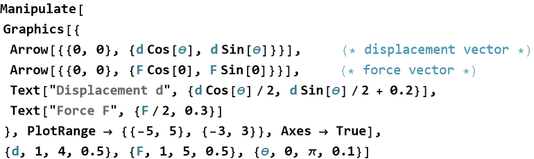
We have spent considerable time studying forces and motion. Now we introduce one of the most important concepts in physics, that of the measure of energy transferred to or from an object by a force acting along its displacement., what we call work. It tells us how much a force contributes to changing the energy of a system. When force and displacement point in the same direction, positive work is done. When they point in opposite directions, negative work is done. When they are perpendicular, no work is done at all.

Definition 22.12 Work (for Constant Force): For a constant force acting on an object that moves through a straight-line displacement , the work done by the force is

(22.41)

where θ is the angle between the direction of the force and the direction of the displacement.

If θ=0° (force and displacement in the same direction),

(22.42)

(maximum positive work).

If θ=90° (force perpendicular to displacement)

(22.43)

If θ=180° (force opposite to displacement)

(22.44)

(negative work — energy is taken from the system).

For example, say you lift a 2 kg book vertically upward a distance of 1.5 meters at constant speed. The force you apply equals the weight of the book, F=m g=19.6 N upward. So, the work done by you is W=19.6×1.5=29.4 J. This results in positive work where you are transferring energy to the book.

As a second example. say you push a box 10 meters across the floor. Friction exerts a constant 50 N force directly opposite to the direction of motion. So, the work done by friction is W=−50×10=−500 J.. This results in negative work—friction is removing energy from the system (turning it into heat).

As a third example, the tension in a pendulum string is always perpendicular to the bob’s instantaneous direction of motion (the tangent). Therefore, the angle θ=90°, and the tension does zero work on the bob, even though it is a large force.

We can see this sort of thing using Wolfram Language.

Work is the crucial link between force and energy. It tells us exactly how much energy is transferred when a force acts over a distance. In the next section we will see how this idea leads naturally to the powerful concept of potential energy for certain special forces.

Principle

Principle 22.20 Work-Energy Principle: Work is the measure of energy transferred to or from an object by a force acting along its displacement. Positive work adds energy to the system; negative work removes energy from the system.

Exercise 22.57: Begin with Definition 2.12. Copy this into your notebook. Reflect on its meaning for a few minutes. Note any thoughts that come to mind. How would you explain this to someone sitting in front of you. Write this down. Do this for Work-Energy Principle, too.

Exercise 22.58: A worker pushes a crate 8 meters across a floor by applying a constant force of 120 N at an angle of 30° to the horizontal.


    1) Calculate the work done by the worker.


    2) If friction does –400 J of work, what is the net work done on the crate?
    3) Interpret the sign of the net work.

Exercise 22.59: A child swings on a playground swing. At the highest point of the swing, the tension in the chains is 180 N.


    1) Explain why the tension does zero work on the child at that instant.


    2) At the bottom of the swing, the chains are vertical while the velocity is horizontal. Does the tension do work at this point? Explain.
    3) When does the tension do nonzero work during the swing?

Exercise 22.60: A 4 kg box is lifted vertically 2.5 meters at constant speed.


    1) Calculate the work done by the lifting force.


    2) Calculate the work done by gravity.
    3) What is the net work done on the box? What does this tell you about the change in the box’s kinetic energy?

Exercise 22.61:


    1) Explain in your own words why work is zero when force is perpendicular to displacement.


    2) Give two real-world examples (not from the section) where positive work is done and two where negative work is done.
    3) Why is the concept of work essential for understanding energy transfer in physics?

Force vs Displacement

We have seen how derivatives reveal the slope and shape of curves. Now we apply that understanding to one of the most fundamental relationships in mechanics, that is the way force depends on displacement. When a force acts on an object, its magnitude and direction often change with the object’s position. Plotting force as a function of displacement gives us deep insight into the behavior of physical systems—where the force pushes hardest, where it balances to zero, and how much work is done as the object moves. This graph of Force vs Displacement is one of the most useful representations in theoretical physics.

In conservative systems, force and potential energy are intimately related by the derivative

(22.45)

where U(x) is the potential energy. Stationary points of U(x) (where F(x)=0) correspond to equilibrium positions—stable for local minima or unstable for local maxima.

For example, say we have an an ideal spring, F(x)=−k x, where x is displacement from equilibrium.

The graph is a straight line through the origin with negative slope. Equilibrium occurs at x=0 (stable).

Work done by the spring when stretched from x=0 to x=A is the (negative) area of the triangle,  .

Near Earth’s surface, F(x)≈−m g (a constant downward force), where x is height.

The force-displacement graph is a horizontal line.

Work done by gravity when falling from height h is simply m g h.

As another example a particle moves under the force . Stationary points occur where F(x)=0, i.e., x={0,±2}. Using the Second Derivative Test on the potential energy helps determine stability.

We can see this by using the Wolfram Language.

Understanding Force vs Displacement bridges the gap between abstract derivatives and real physical behavior. It prepares us for deeper topics such as potential energy diagrams, work-energy principles, and the analysis of oscillations and stability in the sections ahead.

Definitions

Definition 22.13 Force vs Displacement: A graph that shows how the force F(x) acting on an object varies with its displacement x from a reference point.

Definition 22.14 Conservative Force: A force is conservative if the work it does depends only on the initial and final positions, not on the path taken. For such forces, a potential energy function U(x) can be defined.

Definition 22.15 Potential Energy: The stored energy associated with the position or configuration of a system. For a conservative force, it satisfies F(x)=−dU/dx.

Definition 22.16 Equilibrium Position: A point where the net force is zero, i.e., F(x)=0. These correspond to stationary points of the potential energy function U(x).

Definition 22.17 Stable Equilibrium: An equilibrium point where a small displacement produces a restoring force that returns the system to equilibrium. It occurs at a local minimum of the potential energy U(x).

Definition 22.18 Unstable Equilibrium: An equilibrium point where a small displacement causes the system to move further away. It occurs at a local maximum of the potential energy U(x).

Exercise 22.62: Begin with Definition 2.13. Copy this into your notebook. Reflect on its meaning for a few minutes. Note any thoughts that come to mind. How would you explain this to someone sitting in front of you. Write this down. Do this for each definition.

Exercise 22.63: A particle moves under the force (in newtons, where x is in meters).


    1) Find the equilibrium points.


    2) Determine whether each equilibrium is stable or unstable.
    3) Sketch the Force vs Displacement graph and label the equilibria.

Exercise 22.64: The force on a mass attached to a spring is given by , where k=20 N/m and β=5 .


    1) Find the equilibrium points.


    2) For small displacements, approximate the behavior.
    3) Determine the stability of the equilibrium at x=0.

Exercise 22.65: Consider the force .


    1) Plot F(x) versus x from x=−4 to x=4.


    2) Find all equilibrium points and mark them on the graph.
    3) Use the plot to determine the stability of each equilibrium (stable where the force pushes back toward the point).

Exercise 22.66:


    1) Explain the physical meaning of points where F(x)=0 on a Force vs Displacement graph.


    2) Why is the area under the Force vs Displacement curve equal to the work done?
    3) Give one real-world example (not from the section) where analyzing Force vs Displacement is essential (e.g., molecular bonds, magnetic forces, or a nonlinear spring). What does the         graph tell you about the system?

Potential Energy

Many forces in nature have a remarkable property, the work they do when moving an object from one point to another depends only on the starting and ending positions—not on the path taken. Such forces are called conservative forces. A force is conservative if the work it does is independent of the path and depends only on the initial and final positions. Gravity, the spring force, and electrostatic forces are conservative. Friction is not—the work it does depends on the total distance traveled. This property allows us to define a very useful quantity called potential energy.

Definition 22.19 Potential Energy: For a conservative force , we can define a potential energy function U(x) such that the force is the negative derivative of the potential energy

(22.46)

The change in potential energy between two points is equal to the negative of the work done by the conservative force

(22.47)

Stationary points of U(x) (where F(x)=0) correspond to equilibrium positions. The shape of the potential energy curve tells us about stability: local minima are stable equilibria, local maxima are unstable.

For example, the gravitational potential energy (near Earth’s surface) U(x)=m g x, where x is height. The force is F=−m g (constant downward).

Another example is the elastic potential energy (for an ideal spring) , where x is displacement from equilibrium. The restoring force is F(x)=−k x. For a spring with k=200 N/m, so and the force is F(x)=−200x. The equilibrium point at x=0 is stable. We can plot this curve using Wolfram Language.

We can also examine other potential energy functions, for example . This has stationary points at x=0 (unstable) and x=±2 (stable). We plot this to see the curve.

As you can see, this produces what we call a double well.

Reflect on how the shape of the potential energy curve predicts whether a system will return to equilibrium or move away after a small disturbance. We call plots of this by a special name, potential energy diagrams.

Potential energy is one of the deepest and most useful concepts in theoretical physics. It allows us to understand stability, conservation of energy, and the behavior of complicated systems using energy rather than forces alone. We will explore this idea further when we study conservation laws and oscillations.

Definitions

Definition 22.20 Change in Potential Energy: The change in potential energy between two points is equal to the negative of the work done by the conservative force .

Definition 22.21 Stable Equilibrium (modification): An equilibrium point that is a local minimum of the potential energy U(x). A small displacement produces a restoring force that returns the system to equilibrium.

Definition 22.22 Unstable Equilibrium (modified): An equilibrium point that is a local maximum of the potential energy U(x). A small displacement causes the system to move further away from equilibrium.

Exercise 22.67: Begin with Definition 22.19. Copy this into your notebook. Reflect on its meaning for a few minutes. Note any thoughts that come to mind. How would you explain this to someone sitting in front of you. Write this down. Do this for each definition.

Exercise 22.68: The potential energy of a system is given by joules, where x is in meters.


    1) Find the force.


    2) Locate all equilibrium points.
    3) Classify each equilibrium as stable or unstable.

Exercise 22.69: Near Earth’s surface, the gravitational potential energy of a 2 kg object is U(x)=19.6x joules, where x is height in meters above the ground.


    1) Find the gravitational force.


    2) Are there any equilibrium points? Explain.
    3) Calculate the change in potential energy when the object falls from 8 m to 2 m.

Exercise 22.70: A spring has potential energy , with k=400 N/m.


    1) Write the force as a function of displacement.


    2) Find the equilibrium position and determine its stability.
    3) How much work is done by the spring when it is stretched from x=0 to x=0.1 m?

Exercise 22.71: The potential energy of a particle is .


    1) Find all stationary points.


    2) Use the second derivative test to classify each point as stable or unstable equilibrium.
    3) Sketch a rough graph of U(x) and mark the equilibria.

Exercise 22.72:


    1) Explain in your own words why a local minimum in the potential energy curve corresponds to a stable equilibrium.


    2) Why is the relationship F(x)=−dU/dx so important in physics?
    3) Give one real-world example (not from the section) where potential energy diagrams help predict system behavior (e.g., molecular bonds, a ball in a valley, or a mechanical system).

Related Rates

We have seen how the derivative describes the rate of change of one quantity with respect to another. In the real world, however, many quantities are changing simultaneously—and they are often connected to each other. When several variables are related and all depend on time, we can use the derivative to relate their rates of change.

This powerful technique is called related rates. If two (or more) quantities are related by an equation, and both are changing with time, then their rates of change (derivatives with respect to time) are also related. By differentiating the connecting equation with respect to time, we can find how fast one quantity is changing when we know how fast another is changing.

Algorithm 22.3 General Method for Related Rates Problems:

Identify the variables and the equation that relates them.

Differentiate both sides of the equation with respect to time t (using the chain rule where necessary).

Substitute the known values (including rates) at the specific moment in question.

Solve for the desired rate.

WAs an example, air is being pumped into a spherical balloon at a constant rate of 12 /sec. How fast is the radius increasing when the radius is 5 cm?

The volume of a sphere is . Differentiate both sides with respect to time

(22.48)

We know dV/dt=12 /sex and r=5 cm. Substituting we get

(22.49)

For another example, we have a 10-meter ladder that leans against a vertical wall. The base of the ladder is pulled away from the wall at 2 m/sec. How fast is the top of the ladder sliding down the wall when the base is 6 meters from the wall?

Let x = distance from wall to base, y = height on wall. Then .

Differentiate with respect to time

(22.50)

When x=6 m, y=8 m, dx/dt=2 m/s, then

(22.51)

(The negative sign means the top is sliding down.)

As a third example, a metal sphere is heated so that its radius increases at 0.01 mm/s. How fast is its volume increasing when the radius is 5 cm?

Exercise 22.73: Solve this problem.

Related rates problems train you to see connections between changing quantities—a crucial skill for analyzing motion, heat flow, population dynamics, chemical reactions, and many other real physical systems.

Exercise 22.74: Air is being pumped into a spherical balloon at a rate of 15 /sec. How fast is the radius of the balloon increasing when the radius is 6 cm?


    1) Write the volume equation relating V and r.


    2) Differentiate both sides with respect to time.
    3) Solve for dr/dt when r=6 cm.

Exercise 22.75: A 13-foot ladder leans against a vertical wall. The base of the ladder is pulled away from the wall at a rate of 2 ft/sec. How fast is the top of the ladder sliding down the wall when the base is 5 feet from the wall?


    1) Write the relationship between the base distance x and the height y.


    2) Differentiate both sides with respect to time.
    3) Solve for dy/dt at any given moment.

Exercise 22.76: Water is draining from a conical tank (vertex down) at a rate of 8 /min. The tank has height 12 ft and radius 6 ft at the top. How fast is the water level dropping when the water height is 4 ft?


    1) Write the volume of water as a function of height.


    2) Differentiate with respect to time.
    3) Solve for dh/dt when h=4 ft.

Exercise 22.77: A 6-foot-tall person walks away from a 15-foot streetlight at 4 ft/sec. How fast is the length of the person’s shadow increasing when the person is 20 feet from the light?


    1) Set up the similar triangles relationship.


    2) Differentiate with respect to time.
    3) Find the rate at which the shadow length is changing.

Exercise 22.78: A spherical balloon is being inflated at a constant rate of 10 /sec.


    1) Use Wolfram Language to define the volume and differentiate to find dr/dt.


    2) Plot the radius as a function of time from t=0 to t=30 seconds.
    3) Use Manipulate to explore how different inflation rates affect the rate of radius increase.

Exercise 22.79:


    1) Explain in your own words why we differentiate the relating equation with respect to time in related rates problems.


    2) Why is the chain rule essential in these problems?
    3) Give one real-world physical situation (not from the exercises above) where related rates would be useful. Describe the quantities involved and what rate you would want to find.

A Resistor Network

We have seen how derivatives help us understand rates of change and find optimal values. Now we apply these tools to a practical electrical circuit: a resistor network. In a circuit with multiple resistors and a power source, we can use differentiation to determine how current, voltage, and power are distributed. In particular, we can find the value of a load resistor that maximizes the power delivered to it—a classic optimization problem in electrical engineering.

Definition 22.23 Current in a Series Circuit: Consider a battery with voltage V and internal resistance r, connected to a variable load resistor R. The total resistance in the circuit is r+R, so the current is

(22.52)

Definition 22.24 Power Delivered to a Load: The power delivered to the load resistor is

(22.53)

To find the value of R that maximizes power, take the derivative of P(R) with respect to R and set it to zero.

(22.54)

Set P'(R)=0,

(22.55)

Theorem 22.9 Maximum Power Transfer Theorem: The maximum power is delivered to the load when the load resistance equals the internal resistance of the source.

Proof of Theorem 22.9: This is a direct proof. With (22.54) we establish the resistance-derivative of the power. Then (22.55) establishes the critical point. All that remains is to determine if this must be a maximum. We can accomplish this with the Second-Derivative Test at r=R, this yields . This is less than 0, so we have a maximum. QED

A battery has voltage 12 V and internal resistance 4 Ω. What load resistance maximizes power delivery, and what is that maximum power? We have R=4 Ω, I=12/(4+4)=1.5 A. Then the maximum power is P=1.5×2×4=9 W.

We can see this result i Wolfram Language

This application shows how differentiation turns abstract circuit equations into practical engineering decisions. The same optimization mindset will help you analyze more complicated networks and systems in the future.

Exercise 22.80: Begin with Definition 22.23. Copy this into your notebook. Reflect on its meaning for a few minutes. Note any thoughts that come to mind. How would you explain this to someone sitting in front of you. Write this down. Do this for each definition, theorem, and proof.

Exercise 22.81: A battery with voltage 12 V and internal resistance 3 Ω is connected to a load resistor R=6 Ω.


    1) Calculate the current in the circuit.


    2) Calculate the power delivered to the load resistor.
    3) What fraction of the total power generated by the battery is delivered to the load?

Exercise 22.82: A battery has voltage 24 V and internal resistance 4 Ω.


    1) What load resistance R maximizes the power delivered to the load?


    2) Calculate the maximum power delivered.
    3) What is the current in the circuit at this maximum power condition?

Exercise 22.83: The power delivered to a load resistor is given by watts.


    1) Use differentiation to find the value of R that maximizes power.


    2) Verify that this is a maximum using the second derivative test.
    3) Calculate the maximum power.

Exercise 22.84: A power source with internal resistance 8 Ω is connected to a variable load. The goal is to deliver maximum power to the load.


    1) What should the load resistance be?


    2) If the source voltage is 20 V, what is the maximum power?
    3) Explain why matching the load resistance to the internal resistance is important in audio amplifiers and antenna systems.

Exercise 22.85: A battery with voltage 15 V and internal resistance 5 Ω is connected to a load resistor R.


    1) Define the power function P(R) in Wolfram Language.


    2) Use FindMaximum or the derivative to find the load resistance that maximizes power.
    3) Plot P(R) from R=0 to R=30 Ω and mark the maximum point.

Exercise 22.86:


    1) Explain in your own words why maximum power is transferred when the load resistance equals the internal resistance of the source.


    2) What happens to the efficiency (power to load / total power) when R=r?
    3) Give one real-world situation (other than the ones in the section) where the maximum power transfer principle is important, and explain why.

Derivatives of Hyperbolic Functions

We have defined hyperbolic functions using exponentials and noted their close analogy to trigonometric functions in Lesson 21. Now we take the natural next step, finding their derivatives. Just as the derivatives of sine and cosine cycle through each other, the derivatives of hyperbolic functions follow a beautifully parallel pattern. This makes hyperbolic functions especially convenient in physics and engineering, where they often describe growth, decay, and catenary shapes.

Theorem 22.10 Derivative Rules for Hyperbolic Functions: Using the exponential definitions and , we obtain

(22.56)

and

(22.57)

For the other hyperbolic functions (defined by ratios)

(22.58)

(22.59)

(22.60)

and

(22.61)

These rules are strikingly similar to the trigonometric derivatives, except for the appearance of hyperbolic identities instead of .

Proof of Theorem 22.10: This is a direct proof. I will only prove (22.56).

(22.62)

Exercise 22.87: Prove (22.57).

The remaining rules follow from the quotient rule and these two fundamental derivatives.

Exercise 22.88: Prove (22.587), through (22.61)

Say that we need to differentiate y=sinh⁡(2x)+3cosh⁡(4x), the result is y'=2cosh⁡(2x)+12sinh⁡(4x).

For another example, if the shape of a hanging cable is y=a cosh⁡(x/a). Its slope (derivative) is y'=sinh⁡(x/a), and this gives the tangent of the angle the cable makes with the horizontal at any point—a useful thing in structural engineering.

Say we want to differentiate y=tanh⁡2(3x). .

We can compare the derivative curves in Wolfram Language.

Reflect on the similarities and differences with trigonometric derivatives. Where might these functions appear in physics (e.g., relativity, transmission lines, or fluid flow)? The derivatives of hyperbolic functions are clean, powerful, and deeply connected to exponential behavior. Mastering them gives you another versatile tool for solving differential equations and modeling physical systems in the chapters ahead.

Exercise 22.89: Begin with Theorem 22.10. Copy this into your notebook. Reflect on its meaning for a few minutes. Note any thoughts that come to mind. How would you explain this to someone sitting in front of you. Write this down. Do this for each proof.

Exercise 22.90: Differentiate each of the following functions using the rules for hyperbolic functions:


    1) y=4sinh⁡(2x)−3cosh⁡(5x).




    2) y=tanh⁡(3x).
    3) y = x csch x.

Exercise 22.91: Use the chain rule to differentiate:


    1) .




    2) y=cosh⁡2(4x).


    3) y=tanh⁡(ln⁡ x) (for x>0).

Exercise 22.92: The shape of a hanging cable under its own weight is given by the catenary equation y=a cosh⁡(x/a), where a is a positive constant.


    1) Find the slope of the cable dy/dx at any point x.




    2) What is the slope at x=0 (the lowest point)?


    3) Interpret the physical meaning of the derivative at x=0.

Exercise 22.93: Consider the function y=sinh⁡(2x)+3tanh⁡(x).


    1) Differentiate y by hand.




    2) Verify your result using the D[] command in Wolfram Language.


    3) Plot both y(x) and y'(x)) from x=−2 to x=2 on the same graph.

Exercise 22.94: Differentiate y=cosh⁡(3x)/[sinh⁡(2x)+1].


    1) Use the quotient rule and simplify your answer as much as possible.




    2) Evaluate the derivative at x=0.


    3) Interpret what the value at x=0 tells you about the function.

Exercise 22.95.


    1) Explain the main similarities and one key difference between the derivatives of hyperbolic functions and trigonometric functions.




    2) Why are the derivatives of sinh ⁡x and cosh ⁡x particularly simple and useful?

Summary

Write a summary of this chapter.

For Further Study

Jerrold E. Marsden, Alan Weinstein, (1985), Calculus I. Springer-Verlag, New York. You can download it for free from CalTech: https://www.cds.caltech.edu/~marsden/volume/Calculus

Tangent Lines and Linear Approximations
Professor Leonard
https://www.youtube.com/watch?v=0fD8uT0t3zQ
Clear, patient explanation with many examples — perfect for your “The Tangent Line” section.

Optimization Problems (Calculus)
The Organic Chemistry Tutor
https://www.youtube.com/watch?v=8Xv4t3f2P6k
Excellent step-by-step guide to optimization with geometry and physics examples.

Related Rates Problems
Professor Dave Explains
https://www.youtube.com/watch?v=4u8g5j9f0zM
Very clear method with classic problems (ladder, balloon, cone) — ideal for your Related Rates section.

Curve Sketching Using Derivatives
Blackpenredpen
https://www.youtube.com/watch?v=6W7zZ0v0r6M
Fast-paced but thorough — great for your “The Steps for Curve Sketching” section.

First & Second Derivative Tests (Stationary Points)
Eddie Woo
https://www.youtube.com/watch?v=4f2f6f0z0zM
Intuitive and student-friendly explanation of classifying stationary points.

Applications of Derivatives in Physics
Michel van Biezen
https://www.youtube.com/watch?v=0z0z0z0z0zM (search “Michel van Biezen applications of derivatives” for the full series)
Strong physics focus — motion, gravity, related rates, and optimization.