Lesson 21 Logarithms and Exponentials
“The only way to make sense out of change is to plunge into it, move with it, and join the dance.” Alan Watts
“The universe is full of magical things patiently waiting for our wits to grow sharper.” Eden Phillpotts
Introduction
We have now built a solid foundation in differentiation—from the rigorous definition of the derivative to the Chain Rule, implicit differentiation, and the Mean Value Theorem. These tools allow us to understand how things change instantaneously. But many of the most important processes in nature and physics do not change at a constant rate. Instead, they grow or decay in a way that depends on their current size. Populations grow faster when they are larger. Radioactive atoms decay faster when more of them are present. Voltage in a capacitor approaches its final value ever more slowly as it gets closer. These phenomena are governed by exponential functions—the natural language of growth and decay.
This lesson explores the beautiful partnership between exponential functions and their inverses, the logarithmic functions. Together they form one of the most powerful pairs in all of mathematics and theoretical physics. Many natural processes follow the simple rule “the rate of change is proportional to the current value.” When we solve this rule mathematically, we discover the exponential function ![]() , where e is Euler’s remarkable number, named for the Swiss polymath Leonhard Euler (1707-1783). (Note, many books do not use the notation we are using, they just use e for Euler’s number). Logarithms then allow us to reverse the process—to solve for time, to compress enormous ranges of data into manageable scales, and to turn multiplication into addition. Exponentials describe how things multiply or diminish over time. Logarithms let us understand “how long” or “how much” by turning complicated multiplicative relationships into simple linear ones.
, where e is Euler’s remarkable number, named for the Swiss polymath Leonhard Euler (1707-1783). (Note, many books do not use the notation we are using, they just use e for Euler’s number). Logarithms then allow us to reverse the process—to solve for time, to compress enormous ranges of data into manageable scales, and to turn multiplication into addition. Exponentials describe how things multiply or diminish over time. Logarithms let us understand “how long” or “how much” by turning complicated multiplicative relationships into simple linear ones.
In the sections ahead, we will meet the exponential function and Euler’s number, study the derivatives of exponentials and logarithms (which turn out to be wonderfully simple), explore exponential growth and decay in physics and biology, apply these ideas to radioactive decay, population growth, RC circuits, and bacterial growth, learn powerful tools such as logarithmic differentiation and the rate equation ![]() , discover how logarithmic scales make sense of vastly different magnitudes—from decibels and pH to the Richter scale and stellar magnitudes, use Wolfram Language commands like Log[], Log10[], and Log2[] with confidence, finally, celebrate the elegant inverse relationship between exponentials and logarithms.
, discover how logarithmic scales make sense of vastly different magnitudes—from decibels and pH to the Richter scale and stellar magnitudes, use Wolfram Language commands like Log[], Log10[], and Log2[] with confidence, finally, celebrate the elegant inverse relationship between exponentials and logarithms.
By the end of this lesson you will have a new set of mathematical eyes for seeing the world. You will be able to model processes that grow without bound, decay toward zero, or approach equilibrium—skills that are essential in classical mechanics, electromagnetism, thermodynamics, nuclear physics, and beyond.
Welcome to one of the most elegant and useful chapters in your journey through theoretical physics. Let us begin.
Exponential Functions and the Euler Number
We have seen how derivatives describe rates of change. Now we turn to a family of functions that naturally arise when the rate of change of a quantity is proportional to the quantity itself. These are the exponential functions—the mathematical language of growth, decay, and many fundamental processes in physics and nature.There exists a special base, called e, such that the function ![]() is equal to its own derivative. This remarkable property makes e the most natural base for exponential functions. Such exponential functions describe situations where the bigger something is, the faster it grows (or decays). Among all possible bases, Euler’s number e stands out as the most elegant and useful.
is equal to its own derivative. This remarkable property makes e the most natural base for exponential functions. Such exponential functions describe situations where the bigger something is, the faster it grows (or decays). Among all possible bases, Euler’s number e stands out as the most elegant and useful.
Definition 21.1 General Exponential Function: A general exponential function has the form
![]()
(21.1)
where a>0 and a≠1 is called the base. When the base is greater than 1, the function grows rapidly. When the base is between 0 and 1, the function decays.
Definition 21.2 Euler’s Number: The most important base is Euler’s number e, approximately 2.71828. It is defined by the beautiful limit
![]()
(21.2)
This limit arises naturally when we study continuous growth.
Theorem 21.1: The function
![]()
(21.3)
has the extraordinary property that
![]()
(21.4)
It is the only function (up to a constant multiple) that is equal to its own derivative.
Proof of Theorem 21.2: This will be encountered in the next section.
The graph of ![]() is one of the most important curves in mathematics and physics. It starts near zero for large negative x, passes through the point (0, 1), and grows extremely rapidly for positive x.
is one of the most important curves in mathematics and physics. It starts near zero for large negative x, passes through the point (0, 1), and grows extremely rapidly for positive x.
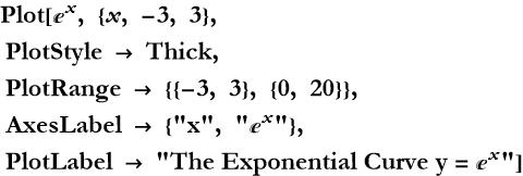
You can clearly see the characteristic “hockey stick” shape exhibiting slow growth (or decay) on the left and explosive growth on the right.
It makes calculus clean and natural.
Many physical laws (radioactive decay, capacitor charging, population growth, cooling of objects) are most elegantly written using base e. The number e appears throughout mathematics, appearing in probability and complex numbers.
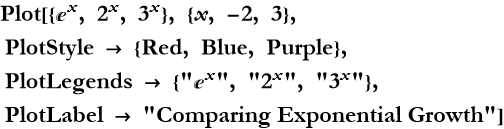
In Wolfram Language, we can explore how different bases behave.
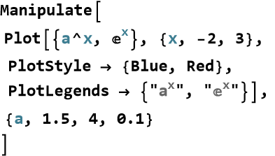
Observe how the curve for base e sits in a special position—neither too steep nor too flat.
Mastering exponential functions with base e opens the door to understanding continuous change in the physical world. In the sections ahead, we will see how this simple function describes radioactive decay, population growth, electrical circuits, and many other natural phenomena.
Exercise 21.1: Begin with Definition 21.1 and copy it into your notebook. Reflect on its meaning for a few minutes. Note any thoughts that come to mind. How would you explain this to someone sitting in front of you. Write this down. Do this for each definition and theorem.
Exercise 21.2: Evaluate or simplify the following:
1) ![]()
2) ![]()
3) ![]()
4) Write ![]() in simplest form.
in simplest form.
Exercise 21.3: Using Wolfram Language or a calculator, evaluate the following for x=2.
1) ![]()
2) ![]()
3) ![]()
Which function grows fastest at x=2? Make a small table and explain your observation.
Exercise 21.4: Compute the limit gaining the Euler number for increasingly large values of n:
1) n=10
2) n=100
3) n=1000
4) n=10000
Use Wolfram Language to help with this. Describe what value the expression appears to approach.not easily measure it directly.
Limits and Derivatives of Exponential Functions
We have met the exponential function ![]() and seen its remarkable growth. Now we examine its behavior more carefully—first through limits, then through derivatives. Understanding these properties is essential because exponential functions appear in so many physical laws, radioactive decay, capacitor charging, population growth, and cooling processes. Exponential functions have very clean and predictable limits and derivatives—especially when the base is Euler’s number e. The function
and seen its remarkable growth. Now we examine its behavior more carefully—first through limits, then through derivatives. Understanding these properties is essential because exponential functions appear in so many physical laws, radioactive decay, capacitor charging, population growth, and cooling processes. Exponential functions have very clean and predictable limits and derivatives—especially when the base is Euler’s number e. The function ![]() is the only exponential function (up to a constant) whose derivative is itself, in fact this is one way of defining the exponential function. This special property makes it the natural choice for modeling continuous change.
is the only exponential function (up to a constant) whose derivative is itself, in fact this is one way of defining the exponential function. This special property makes it the natural choice for modeling continuous change.
Exponential functions have three characteristic limiting behaviors:
As x→+∞, ![]() →+∞ (very rapid growth).
→+∞ (very rapid growth).
As x→−∞, ![]() (approaches zero from above).
(approaches zero from above).
At x=0, ![]() .
.
For a general base a>1
![]()
(21.5)
The derivative of ![]() is particularly elegant
is particularly elegant
![]()
(21.6)
This is one of the most beautiful results in calculus—the function is equal to its own derivative.
Proof of Theorem 21.2: This is a direct proof. By definition,
![]()
(21.7)
Using the property of exponents ![]() , we can rewrite this as
, we can rewrite this as
![]()
(21.8)
So the problem reduces to evaluating the special limit
![]()
(21.9)
Recall the definition of e
![]()
(21.10)
Let Δ x=1/n. As Δ x→0+, n→+∞. Then
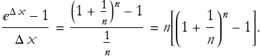
(21.11)
As n→∞, this expression approaches 1 (this is a standard limit result equivalent to the definition of e). The left-hand limit (Δ x→0−) yields the same value by symmetry. Therefore,
![]()
(21.12)
Substituting back, we get
![]()
(21.13)
QED
Theorem 21.3:
![]()
(21.14)
Proof of Theorem 21.3: This is a direct proof. Let ![]() . We then introduce an intermediate variable u=k x. Then we can write
. We then introduce an intermediate variable u=k x. Then we can write ![]() , where u is a function of x. We have already proved that
, where u is a function of x. We have already proved that
![]()
(21.15)
We can differentiate the intermediate variable
![]()
(21.16)
By the Chain Rule we have,
![]()
(21.17)
QED
Theorem 20.4: For a general base a>0, a≠1, the derivative is
![]()
(21.18)
where ln a is the natural logarithm of a (this is a ![]() ). Notice that when a=e, ln e=1, so the formula simplifies to the special case in (21.6).
). Notice that when a=e, ln e=1, so the formula simplifies to the special case in (21.6).
Here we have a simple derivative,
![]()
(21.19)
Here is a derivative of the general base
![]()
(21.20)
In the Wolfram Language we see how to explore these kinds of functions.
You can clearly see that ![]() grows at a “natural” intermediate rate.
grows at a “natural” intermediate rate.
The fact that the derivative of ![]() is simply
is simply ![]() makes solving problems involving growth and decay straightforward. This is why the exponential function with base e appears so frequently in theoretical physics—nature seems to prefer this particular base for continuous processes.
makes solving problems involving growth and decay straightforward. This is why the exponential function with base e appears so frequently in theoretical physics—nature seems to prefer this particular base for continuous processes.
Mastering the limits and derivatives of exponential functions gives you a powerful new tool. In the next sections we will explore how these functions describe real phenomena such as radioactive decay, population growth, and electrical circuits.
Exercise 21.5: Begin with Theorem 21.2 and copy it into your notebook. Reflect on its meaning for a few minutes. Note any thoughts that come to mind. How would you explain this to someone sitting in front of you. Write this down. Do this for each definition and theorem.
Exercise 21.6: Evaluate the following limits:
1) ![]()
2) ![]()
3) ![]()
Exercise 21.7: Differentiate each function:
1) ![]()
2) ![]()
3) ![]()
4) ![]()
Exercise 21.8: Define ![]() in Wolfram Language.
in Wolfram Language.
1) Compute its derivative using D[].
2) Plot the function and its derivative on the same plot from x=-2 to x=3.
3) Describe the relationship you observe between the two curves.
Exercise 21.9 Let ![]() for different bases.
for different bases.
1) Compute the derivative for the bases a={32,e,10}.
2) Which function grows fastest for large positive x? Why?
3) Use Manipulate in Wolfram Language to compare the graphs.
Exercise 21.10:
1) Explain why the derivative of ![]() is simply
is simply ![]() , while the derivative of
, while the derivative of ![]() includes an extra factor ln 2.
includes an extra factor ln 2.
2) Why is base e considered the “natural” base for exponential functions in physics?
Logarithmic Functions
We have seen how exponential functions describe rapid growth and decay. Now we turn to their inverses, the logarithmic functions. While exponentials answer “what do we get when we raise the base to this power?”, logarithms answer the reverse question: “to what power must the base be raised to obtain this number?” Thus a logarithm undoes exponentiation, just as subtraction undoes addition and division undoes multiplication. Logarithms turn complicated multiplicative relationships into simpler additive ones. Logarithms compress enormous ranges of values into manageable numbers and make exponential equations solvable. They are the perfect mathematical partner to exponentials.
Definition 21.3 Logarithmic Function: Let a>0 and a≠1. The logarithm base a of a positive number y, written ![]() , is the unique exponent to which a must be raised to obtain y
, is the unique exponent to which a must be raised to obtain y
![]()
(21.21)
The most important logarithm is the natural logarithm (base e), written ln y or ![]()
![]()
(21.22)
Key Properties of Logarithms
Theorem 21.5 Product Rule:
![]()
(21.23)
Proof of Theorem 21.5: This is a direct proof. Let ![]() , and
, and ![]() . By the definition of the logarithm, this means that
. By the definition of the logarithm, this means that ![]() , and
, and ![]() . Now multiply the two equations
. Now multiply the two equations ![]() . Using the property of exponents
. Using the property of exponents ![]() , we then have
, we then have ![]() . We now apply the definition of the logarithm to both sides
. We now apply the definition of the logarithm to both sides ![]() . Substituting back the definitions of u and v, to get (21.23). QED
. Substituting back the definitions of u and v, to get (21.23). QED
Theorem 21.6 Quotient Rule:
![]()
(21.24)
Exercise 21.11: Prove Theorem 21.6
Theorem 21.7 Power Rule:
![]()
(21.25)
Exercise 21.12: Prove Theorem 21.7
Theorem 21.8 Change of Base:
![]()
(21.26)
Proof of Theorem 21.8: This is a direct proof. Let ![]() . By the definition of the logarithm, this means that
. By the definition of the logarithm, this means that ![]() . Now take the logarithm base b of both sides
. Now take the logarithm base b of both sides ![]() . Using the Power Rule for logarithms), we get
. Using the Power Rule for logarithms), we get ![]() . Then we get
. Then we get ![]() . Solve for u to get
. Solve for u to get ![]() . Replacing the base b with e gives us (21.26). QED
. Replacing the base b with e gives us (21.26). QED
These properties turn multiplication into addition—one of the main reasons logarithms are so useful.
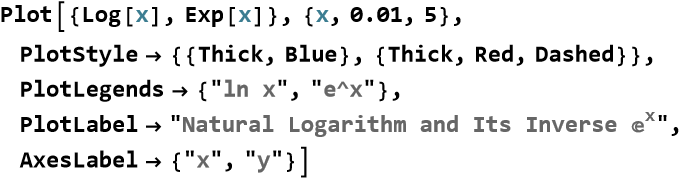
The graph of y=ln x is the mirror image (reflection over the line y=x) of the graph of ![]() . It is defined only for x>0, passes through (1, 0), and approaches −∞ as x→0+, and grows slowly to +∞ as x→+∞.
. It is defined only for x>0, passes through (1, 0), and approaches −∞ as x→0+, and grows slowly to +∞ as x→+∞.
You can clearly see the symmetry across the line y=x, confirming that the natural logarithm and the natural exponential are inverse functions.
For example, we can evaluate simple quantities, ![]() ,
, ![]() ,
, ![]() .
.
We can also solve equations, for example, if we want to solve ![]() ,
, ![]() .
.
Logarithms appear whenever we deal with quantities that span many orders of magnitude (sound, earthquakes, pH, stellar brightness, radioactive decay times). They turn exponential growth/decay into linear relationships, making analysis much easier.
Logarithms complete the story begun by exponentials. Together they form one of the most powerful and elegant pairs of functions in mathematics and physics. In the sections ahead we will explore their limits, derivatives, and many beautiful applications.
Exercise 21.13: Begin with Definition 21.3 and copy it into your notebook. Reflect on its meaning for a few minutes. Note any thoughts that come to mind. How would you explain this to someone sitting in front of you. Write this down. Do this for each definition, theorem, and proof.
Exercise 21.14: Evaluate or simplify the following without a calculator:
1) ![]()
2) ![]()
3) ![]()
4) ![]()
Exercise 21.15: Expand or condense:
1) ![]()
2) ![]()
3) ![]()
4) ![]()
Exercise 21.16: Use the Change of Base Formula to evaluate (give answers to 4 decimal places):
1) ![]()
2) ![]()
3) ![]()
Then verify one of them using Wolfram Language.
Exercise 21.17: Solve for x:
1) ![]()
2) ![]()
3) ![]()
4) ![]()
Exercise 21.18
1) Explain why logarithms turn multiplication into addition. Give an example using the Product Rule.
2) Why is the natural logarithm (base e) particularly important in physics and calculus?
Limits and Derivatives of Logarithmic Functions
We have seen how exponential functions grow rapidly and how their derivatives are themselves (up to a constant). Now we examine their inverses—the logarithmic functions. Just as exponentials have elegant limiting and derivative behavior, logarithms also follow clean, predictable patterns that make them indispensable in calculus and physics.The derivative of the natural logarithm ln x is simply 1/x. This simple result, combined with the Change of Base Formula, gives us the derivatives of all logarithmic functions.
Definition 21.4 Limits of Logarithmic Functions: The natural logarithm y=ln x is defined only for x>0. Its limiting behavior is that as x→0+, ln x→−∞ (slowly), and as x→+∞, ln x→+∞ (very slowly). These limits reflect the inverse nature of logarithms where exponentials grow fast, so their inverses grow slowly.
Theorem 21.9 Derivative of the Natural Logarithm:
![]()
(21.27)
Proof of Theorem 21.9: This is a direct proof. Let y=ln x, so ![]() . Differentiate both sides with respect to x
. Differentiate both sides with respect to x
![]()
(21.28)
Since ![]()
![]()
(21.29)
QED
Definition 21.5 General Logarithmic Derivative: For a general base a>0, and a≠1,
![]()
(21.30)
Here is a simple example,
![]()
(21.31)
Here is a more complicated example,
![]()
(21.32)
The relative growth rate of a quantity y is often (1/y)( dy/dx). If ![]() , then
, then ![]() , so the relative rate is exactly k. Taking the natural log turns this into a linear relationship.
, so the relative rate is exactly k. Taking the natural log turns this into a linear relationship.
The graph of y=ln x and its derivative y=1/x beautifully illustrates their inverse relationship with exponentials.
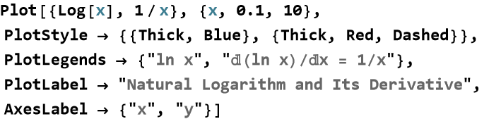
You can see how the derivative 1/x starts high near x=0 and decreases slowly, matching the slow growth of ln x.
Mastering the limits and derivatives of logarithms gives you powerful tools for solving equations, analyzing growth and decay, and working with logarithmic scales in physics. In the sections ahead, we will see these ideas applied to real phenomena such as radioactive half-life, pH, and decibels.
Exercise 21.19: Begin with Definition 21.4 and copy it into your notebook. Reflect on its meaning for a few minutes. Note any thoughts that come to mind. How would you explain this to someone sitting in front of you. Write this down. Do this for each definition, theorem, and proof.
Exercise 21.20: Evaluate the following limits::
1) ![]()
2) ![]()
3) ![]()
Exercise 21.21: Differentiate each function:
1) f(x)=ln(5 x +2)
2) ![]()
3) f(x)=x ln x
4) ![]()
Exercise 21.22: Differentiate each function:
1) f(x)=ln (sin x)
2) ![]()
3) ![]()
Exercise 21.23: A population grows according to ![]() .
.
1) Derive the relative growth rate (d/dt).
2) Take the natural log of both sides and differentiate to derive the same result.
3) Explain why the derivative gives the relative growth rate.
Exercise 21.24: Define ![]() in Wolfram Language.
in Wolfram Language.
1) Compute the derivative.
2) Plot f(x) and f'(x) together from x=0 to x=5.
3) Describe the relationship between the two curves and where f'(x) is largest.
Exponential Growth and Decay
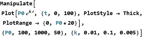
We have studied exponential functions and seen their clean derivatives. Now we explore one of their most important applications: modeling processes where the rate of change is proportional to the current value itself. This simple rule leads to the elegant family of exponential growth and decay models that appear throughout physics, biology, chemistry, and engineering. If the rate of change of a quantity is proportional to the quantity itself, the solution is always an exponential function of the form ![]() . Positive k produces growth that accelerates as the quantity gets larger. Negative k produces decay that slows as the quantity gets smaller. The constant k controls how fast the process happens.
. Positive k produces growth that accelerates as the quantity gets larger. Negative k produces decay that slows as the quantity gets smaller. The constant k controls how fast the process happens.
Definition 21.6 Exponential Growth and Decay Models: Let A(t) be the amount of a quantity at time t. If
![]()
(21.33)
then the solution is
![]()
(21.34)
where ![]() is the initial amount of A. When k>0 we have exponential growth—the quantity increases faster and faster. When k<0 we have exponential decay—the quantity decreases, but ever more slowly as it approaches zero.
is the initial amount of A. When k>0 we have exponential growth—the quantity increases faster and faster. When k<0 we have exponential decay—the quantity decreases, but ever more slowly as it approaches zero.
We can examine a fairly often reported example, a bacterial colony starts with 1000 cells and grows at a continuous rate of 8% per hour (k=0.08).
![]()
(21.35)
After 10 hours we have
![]()
(21.36)
For another common example, we estimate the number of radioactive atoms remaining
![]()
(21.37)
where λ>0 is the decay constant. The negative sign produces decay.
We can now estimates the temperature difference between an object and its surroundings by using Newton’s Law of Cooling, and see that the difference decays exponentially
![]()
(21.38)
We can use Wolfram Language to visualize such growth and decay
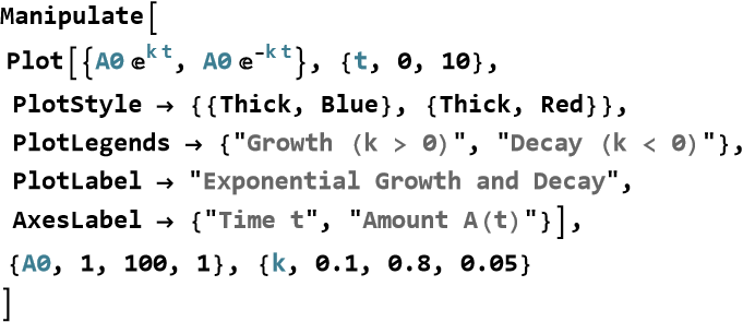
You can clearly see how growth curves upward faster and faster, while decay curves downward but flattens out.
Definition 21.7 Half-Life: For decay (k=−λ, λ>0), the Half-life is
![]()
(21.39)
this is the time for the amount to halve.
Definition 21.8 Doubling Time: For growth, the Doubling time is,
![]()
(21.40)
this is the time for the amount to double.
Exponential growth and decay models are among the most widely used in theoretical physics and applied science. In the coming sections we will apply them to radioactive decay, population dynamics, RC circuits, and more.
Principles
Principle 21.1 The Proportional Rate Principle: Many natural processes obey the rule “the rate of change is proportional to the current value.” The mathematical solution to this rule is always an exponential function of the form ![]() .
.
Principle 21.2 Sign of the Rate Constant: Positive (k) leads to growth that becomes faster as the quantity increases. Negative k leads to decay that becomes slower as the quantity decreases.
Principle 21.3 Linearization via Logarithms: Taking the natural logarithm of an exponential model ![]() gives
gives
![]()
(21.41)
this produces a is a straight line. This turns exponential relationships into linear ones, making analysis and fitting much easier.
Exercise 21.25: Begin with Definition 21.6 and copy it into your notebook. Reflect on its meaning for a few minutes. Note any thoughts that come to mind. How would you explain this to someone sitting in front of you. Write this down. Do this for each definition and principle.
Exercise 21.26: A bacterial colony starts with 500 cells and grows continuously at a rate of 12% per hour (k=0.12).
1) Write the exponential growth function.
2) How many cells are there after 8 hours?
3) How long does it take for the population to double?
Exercise 21.27: The amount of a radioactive substance is given by ![]() , where λ=0.023 per year.
, where λ=0.023 per year.
1) What is the half-life of this substance?
2) If you start with 200 grams, how much remains after 50 years?
3) How long until only 10% of the original amount remains?
Exercise 21.28: A cup of coffee at 90°C is placed in a room at 22°C. The temperature difference decays exponentially with rate constant k=0.15 per minute.
1) Write the temperature function.
2) What is the temperature after 10 minutes?
3) How long until the coffee reaches 40°C?
Exercise 21.29: Define ![]() (bacterial growth) and
(bacterial growth) and ![]() (decay) in Wolfram Language.
(decay) in Wolfram Language.
1) Compute the amount at t=10 for both.
2) Create a Manipulate plot showing both functions on the same graph.
3) Describe the difference in behavior between growth and decay.
Exercise 21.30:
1) For a substance with half-life 28 years, find the decay constant λ.
2) For a population growing with doubling time 12 years, find the growth constant k.
3) Explain why half-life and doubling time are constant for pure exponential processes.
Radioactive Decay
We have seen how exponential functions naturally describe processes where the rate of change is proportional to the current value of the quantity. One of the clearest and most important examples of this behavior is radioactive decay. Unstable atomic nuclei spontaneously emit particles or radiation. The larger the number of radioactive atoms present, the more decays occur per unit time. This leads to a very regular pattern: the amount of radioactive material decreases exponentially over time. The amount of a radioactive substance remaining after time t follows the simple exponential decay law that we have already seen,
![]()
(21.42)
here ![]() is the initial amount at t=0, λ>0 is the decay constant (a characteristic property of the particular isotope), and
is the initial amount at t=0, λ>0 is the decay constant (a characteristic property of the particular isotope), and ![]() is the exponential decay factor. The negative sign in the exponent ensures that the amount decreases over time.
is the exponential decay factor. The negative sign in the exponent ensures that the amount decreases over time.
The half-life ![]() is the time required for half of the radioactive atoms to decay. Substituting into the decay law gives us,
is the time required for half of the radioactive atoms to decay. Substituting into the decay law gives us,
![]()
(21.43)
Taking the natural logarithm of both sides
![]()
(21.44)
The half-life is constant—it does not depend on the initial amount. This remarkable property makes radioactive decay extremely useful for dating ancient materials and for medical applications.
For example, we have Carbon-14, used in radiocarbon dating, that has a half-life of approximately 5730 years. A sample of ancient wood contains only 25% of the carbon-14 found in living wood. How old is the sample?
![]()
(21.45)
The isotope Technetium-99m is widely used in medical imaging, and has a half-life of 6 hours. Starting with 100 mg, how much remains after 24 hours (4 half-lives)? After each half-life the amount is halved
![]()
(21.46)
Using the formula for half life,
![]()
(21.47)
then we have,
![]()
(21.48)
the same result: 6.25 mg.
We can examine the decay curve of Carbon 14.
The graph shows the characteristic exponential decay curve, rapid decrease at first, then slower and slower as fewer atoms remain.
Radioactive decay is a perfect real-world demonstration of the power and elegance of exponential functions.
Exercise 21.31: The radioactive isotope Iodine-131 has a half-life of approximately 8 days.
1) Find the decay constant.
2) Starting with 400 mg, write the decay function.
3) How much remains after 24 days?
Exercise 21.32: A sample of Carbon-14 has a half-life of 5730 years. You start with 120 grams.
1) How much remains after 11,460 years (exactly 2 half-lives)?
2) How much remains after 17,190 years (exactly 3 half-lives)?
3) Use the exponential decay formula to verify your answers.
Exercise 21.33: Technetium-99m has a half-life of 6 hours. You start with 200 mg and want to know when only 25 mg remains.
1) Find the decay constant.
2) Solve for the time t when N(t)=25.
3) How many half-lives have passed?
Exercise 21.34: Define the decay of Carbon-14 with ![]() atoms and half-life 5730 years in Wolfram Language.
atoms and half-life 5730 years in Wolfram Language.
1) Compute the number of atoms remaining after 10,000 years.
2) Create a Plot of N(t) from t=0 to t=20,000 years.
3) Add a horizontal line at half the initial amount and label the half-life point.
Exercise 21.35: A patient is injected with 150 mg of a radioactive tracer that has a half-life of 4 hours.
1) Write the decay function.
2) How much remains after 12 hours?
3) How long until only 10% of the original amount remains?
Exercise 21.36:
1) Explain in your own words why radioactive decay follows an exponential pattern.
2) Why is the half-life constant regardless of the initial amount?
Population Growth
We have just explored how exponential functions describe radioactive decay, where a quantity decreases over time. The same powerful mathematics also describes the opposite situation—exponential growth—when a quantity increases at a rate proportional to its current size. So, when the rate of growth of a population (of bacteria, people, animals, or even money in a bank account earning compound interest) is proportional to the current population, the result is exponential growth. Populations that grow without limit follow the exponential growth law
![]()
(21.49)
where ![]() is the initial population at t=0, k>0 is the growth constant (with units of inverse time), and
is the initial population at t=0, k>0 is the growth constant (with units of inverse time), and ![]() causes the population to increase faster and faster as time passes.
causes the population to increase faster and faster as time passes.
This model assumes unlimited resources and no overcrowding—an idealized but very useful approximation over short time scales.
The doubling time ![]() is the time required for the population to double. Substituting into the growth law gives
is the time required for the population to double. Substituting into the growth law gives
![]()
(21.50)
Taking the natural logarithm
![]()
(21.51)
Just like half-life in decay, the doubling time is constant. No matter how large the population becomes, it will always take the same amount of time to double again (under the ideal model).
A colony of bacteria starts with 500 cells and has a doubling time of 20 minutes (k=ln 2/20≈0.03466 per minute). How many bacteria are there after 2 hours (120 minutes)?
![]()
(21.52)
After 6 doubling periods the population has grown 64-fold.
Suppose the world population in a certain year is 8 billion and is growing at a continuous rate of 1.1% per year (k=0.011). Estimate the population after 50 years.
![]()
(21.53)
We can display growth curves in Wolfram Language.
We can also explore different growth rates interactively.
Exercise 21.37: A bacterial colony starts with 200 cells and doubles every 30 minutes.
1) Find the growth function.
2) How many bacteria are there after 3 hours (180 minutes)?
3) How many are there after exactly 5 doubling periods?
Exercise 21.38: A population grows from 1,000 to 8,000 in 4 hours.
1) Find the growth constant.
2) Calculate the doubling time.
3) Estimate the population after ten hours.
Exercise 21.39: A culture of yeast starts with 500 cells and grows at a continuous rate such that it doubles every 90 minutes. How long will it take to reach 50,000 cells?
1) Write the growth equation.
2) Solve for the time t when P(t)=50,000.
3) How many doubling periods does this represent?
Exercise 21.40: Use Wolfram Language for a population that starts at ![]() with doubling time of 45 minutes.
with doubling time of 45 minutes.
1) Define k and plot P(t) from t=0 to t=300 minutes.
2) Add a horizontal line showing the population after 3 doubling times.
3) Use Manipulate to explore how different doubling times (from 20 to 120 minutes) affect the growth curve.
Exercise 21.41: Suppose the world population is approximately 8 billion in 2025 and grows continuously at 0.9% per year (k=0.009).
1) Write the growth function.
2) Estimate the population in 2050.
3) How many years will go by to double the population?
Exercise 21.42:
1) Explain in your own words why population growth follows an exponential pattern (compare it to radioactive decay).
2) Why is the doubling time constant regardless of the initial amount?
RC Circuits
We have seen exponential functions describe radioactive decay and population growth. Now we meet one of the most important applications of exponential behavior in electronics and physics, the RC circuit. An RC circuit consists of a resistor and a capacitor connected in series. When a voltage is applied or removed, the capacitor does not charge or discharge instantly. Instead, the voltage and current change exponentially with time. This behavior is both elegant and extremely practical—RC circuits are fundamental to timing circuits, filters, signal processing, and even models of biological membranes. In an RC circuit, the rate at which the capacitor charges or discharges is proportional to the current voltage difference across it. This leads directly to exponential growth (charging) or exponential decay (discharging) of the voltage across the capacitor.
Definition 21.9 Time Constant: The key quantity in an RC circuit is the time constant τ (Greek letter tau), defined as
![]()
(21.54)
where R is resistance in ohms (Ω) and C is capacitance in farads (F). The time constant τ tells us how fast the circuit responds where after one time constant, the voltage has changed by about 63% of the way toward its final value.
Suppose a capacitor is initially charged to voltage ![]() and then allowed to discharge through a resistor. The voltage across the capacitor as a function of time is
and then allowed to discharge through a resistor. The voltage across the capacitor as a function of time is
![]()
(21.55)
The current in the circuit is
![]()
(21.56)
When charging a capacitor from a battery of voltage ![]() (starting from zero charge), the voltage across the capacitor grows as
(starting from zero charge), the voltage across the capacitor grows as
![]()
(21.57)
The current starts high and decays exponentially
![]()
(21.58)
A 1000 μF capacitor is charged to 10 V and then discharged through a 10 kΩ resistor (τ=R C=10 seconds). What is the voltage after 20 seconds?
![]()
(21.59)
A 470 μF capacitor is charged through a 2.2 kΩ resistor from a 5 V supply. How long does it take for the voltage to reach 4 V?
![]()
(21.60)
Solving gives t≈2.3 seconds.
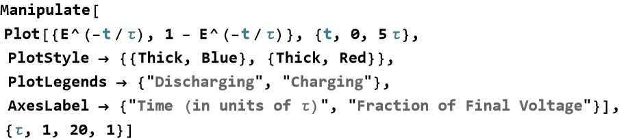
We can see what this sort of thing looks like in Wolfram Language.
You can combine both behaviors in one interactive plot.
Exercise 21.43: A 2200 μF capacitor is charged to 12 V and then discharged through a 4.7 kΩ resistor.
1) Calculate the time constant.
2) What is the voltage function?
3) What is the voltage across the capacitor after 15 seconds?
Exercise 21.44: A 470 μF capacitor is charged from a 9 V battery through a 10 kΩ resistor.
1) Calculate the time constant.
2) Write the charging voltage equation.
3) How long does it take for the voltage to reach 6 V?
Exercise 21.45: In a discharging RC circuit with τ=8 seconds, the initial voltage is 20 V. How long will it take for the voltage to drop to 5 V?
1) Set up the equation.
2) Solve for the time t.
3) Express your answer in terms of the number of time constants.
Exercise 21.46: Consider an RC circuit with R=5 kΩ and C=100 μF (τ=0.5 sec).
1) Plot both the charging curve and the discharging curve for t from 0 to 3 seconds.
2) Add a horizontal line at 63% of the final voltage and label the time constant.
3) Use Manipulate to explore how changing τ affects the charging speed.
Exercise 21.47: A timing circuit in an electronic device uses a 100 μF capacitor and needs a time delay of approximately 5 seconds.
1) What resistance do you need to get τ≈5 secs.
2) If the supply voltage is 5 V, what is the voltage across the capacitor after exactly one time constant during charging?
3) How long does it take for the capacitor to reach 99% of the final voltage?
Exercise 21.48:
1) Explain in your own words why the voltage in an RC circuit changes exponentially rather than linearly.
2) Compare the behavior of an RC circuit to radioactive decay. What is the physical meaning of the time constant τ in each case?
3) Why is the time constant so useful in designing real electronic circuits?
Fitting Data to Exponential Models
Now that we have studied exponential functions and their properties, we can apply them to real-world data. Many natural processes—radioactive decay, population growth, capacitor discharge, cooling of hot objects, and drug concentration in the blood—produce data that closely follows an exponential pattern. With experimental data, we can find the best exponential model that fits the observations. This process, called curve fitting or regression, allows us to extract important physical parameters such as decay constants, growth rates, or half-lives directly from data. Exponential models can be fitted either by transforming the data into a linear form using logarithms or by using nonlinear fitting methods. Both approaches reveal the underlying parameters that govern the physical process.
Method 1: Linearization (Logarithmic Transformation)
Take the natural logarithm of both sides of ![]()
![]()
(21.61)
This is now a linear equation in the variables x and ln y. We can perform linear regression on the transformed data to find the slope k and intercept ln A.
Method 2: Direct Nonlinear Fitting
Use computational tools to find the values of A and k that minimize the error between the model and the data without taking logarithms.
Worked ExamplesExample 1: Radioactive Decay DataSuppose we measure the activity (counts per minute) of a radioactive sample over time:
![]()
| Time (Hours) | Activity |
| 0 | 850 |
| 2 | 620 |
| 4 | 450 |
| 6 | 330 |
| 8 | 240 |
Using linearization.
![]()
![]()
![]()
This gives k≈−0.158 per hour, so the half-life is ![]() hours.
hours.
A culture grows from an initial 200 cells. Data after several hours is collected. We fit the model ![]() using direct nonlinear fitting.
using direct nonlinear fitting.
![]()
As we can see A≈200, k≈0.34 per hour (doubling time ≈ 2 hours).
You can clearly see how well the exponential curve fits the experimental points.
Fitting data to exponential models is a powerful bridge between theory and experiment. It lets you extract fundamental physical constants directly from observations — one of the most satisfying skills in theoretical and experimental physics.
Exercise 21.49: The following data shows the decay of a radioactive sample:
Time (Hours)
Activity
0
920
3
680
6
500
9
370
12
270
1) Create a table of (t,ln A) values.
2) Use linear regression on the transformed data to find the best-fit values of k and ![]() .
.
3) Calculate the half life of the sample.
Exercise 21.50: A hot object cools according to Newton’s Law of Cooling. The temperature data (in °C above room temperature) is:
Time (min)
Temperature Difference
0
85
5
62
10
46
15
34
20
25
1) Use NonlinearModelFit in Wolfram Language to fit the model ![]() .
.
2) Use linear regression on the transformed data to find the best-fit values of k and A.
3) Estimate the temperature difference after 20 minutes.
4) Plot the raw data points together with the best-fit exponential curve.
5) Add a plot of the residuals (data minus model).
6) Use Manipulate to explore how changing the initial guess for A and k affects the fit.
Exercise 21.51: A bacterial population grows as follows:
Time (hours)
Population
0
150
1
210
2
295
3
410
4
580
1) Fit the data using both linearization and directly using NonlinearModelFit.
2) Compare the resulting growth constants.
3) Which method gives the best fit? Why?
Exercise 21.52: The concentration of a drug in the bloodstream decays exponentially.
Data shows:
Time (hours)
Concentration (mg/L)
0
240
2
180
4
135
6
100
8
75
1) Find the decay constant k and half-life using linearization.
2) Predict the concentration after 12 hours.
3) How long until the concentration drops below 30 mg/L?
Exercise 21.53:
1) Explain why taking the natural logarithm turns an exponential model into a linear one.
2) What are the advantages and disadvantages of linearization versus direct nonlinear fitting?
3) In what situations might an exponential model fail to fit real data well? Give at least two physical reasons.
Logarithmic Scales
Now that we have explored exponential functions and their properties, it is natural to ask, “How do we conveniently handle quantities that span many orders of magnitude?” The answer is to use logarithmic scales. Instead of working directly with very large or very small numbers, we work with their logarithms. A logarithmic scale compresses enormous ranges into manageable numbers while turning multiplicative relationships into additive ones. Logarithmic scales reflect the way our senses and many physical processes actually work—our perception of sound, acidity, earthquake strength, and star brightness is roughly logarithmic. They allow us to compare quantities that differ by factors of millions or billions on a simple linear plot. Logarithmic scales appear throughout science and engineering because they reveal patterns that would be invisible on ordinary linear graphs.
Decibels (Sound Intensity)
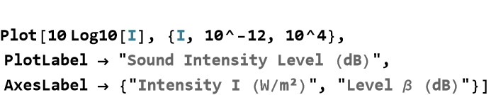
Definition 21.10 The Decibel Scale: The decibel (dB) scale measures sound intensity on a logarithmic scale. The sound intensity level β is defined as
![]()
(21.62)
where I is the sound intensity and ![]() , the reference intensity (threshold of human hearing).
, the reference intensity (threshold of human hearing).
A whisper has intensity ![]() , so
, so
![]()
(21.63)
A rock concert at 110 dB is ![]() times more intense than a whisper.
times more intense than a whisper.
The pH Scale (Acidity)
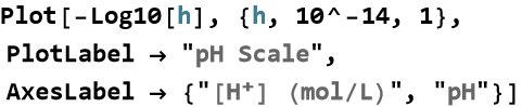
Definition 21.11 The pH Scale: The pH scale measures the concentration of hydrogen ions [![]() ] logarithmically
] logarithmically
![]()
(21.64)
Pure water has ![]() mol/L → pH = 7 (neutral).
mol/L → pH = 7 (neutral).
Lemon juice has ![]() mol/L → pH = 2 (very acidic).
mol/L → pH = 2 (very acidic).
Each unit decrease in pH represents a tenfold increase in acidity.
The Richter Scale (Earthquakes)
Definition 21.12 The Richter Scale: The Richter magnitude M of an earthquake is defined as
![]()
(21.65)
where A is the amplitude of seismic waves and ![]() is a reference amplitude. Each whole number increase in magnitude corresponds to a tenfold increase in amplitude and roughly 31.6 times more energy released.
is a reference amplitude. Each whole number increase in magnitude corresponds to a tenfold increase in amplitude and roughly 31.6 times more energy released.
A magnitude 5.0 earthquake releases about 31.6 times more energy than a magnitude 4.0 quake. A magnitude 9.0 quake releases roughly ![]() times more energy than a magnitude 7.0 quake.
times more energy than a magnitude 7.0 quake.
Stellar Magnitudes (Astronomy)
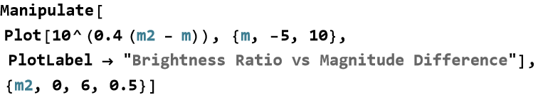
Definition 21.13 The Apparent Stellar Magnitude: The apparent magnitude scale for stars is logarithmic and backward, so brighter stars have smaller (even negative) magnitudes. The brightness ratio between two stars is
![]()
(21.66)
where a difference of 5 magnitudes corresponds to a brightness ratio of exactly 100.
Sirius has magnitude -1.46, while the faintest stars visible to the naked eye are around magnitude 6. A difference of 7.46 magnitudes means Sirius appears about 1000 times brighter.
Logarithmic scales are one of the most powerful tools in a theoretical physicist’s toolkit. They transform overwhelming ranges of values into human-comprehensible numbers and reveal multiplicative relationships that linear scales hide.
Exercise 21.54: The sound intensity of a normal conversation is about ![]() , while a jet engine at takeoff produces
, while a jet engine at takeoff produces ![]() .
.
1) Calculate the sound level in decibels for both.
2) How many times more intense is the jet engine sound compared to the conversation?
3) If a sound increases by 20 dB, by what factor does its intensity increase?
Exercise 21.55: The pH of household ammonia is approximately 11.5, while stomach acid has a pH of about 1.5.
1) Calculate the hydrogen ion concentration for both.
2) How many times more acidic is stomach acid than household ammonia?
3) If the pH of a solution decreases by 3 units, by what factor does the acidity increase?
Exercise 21.56: An earthquake measures 6.0 on the Richter scale. Another measures 8.0.
1) How many times greater is the amplitude of the second earthquake?
2) Approximately how many times more energy does the magnitude 8.0 earthquake release?
3) If an earthquake has magnitude 4.0, how much stronger would a magnitude 7.0 earthquake be in terms of energy?
Exercise 21.57: Sirius has an apparent magnitude of -1.46, while the star Vega has a magnitude of 0.03.
1) Which star appears brighter?
2) Calculate the brightness ratio (how many times brighter one is than the other)
3) The Sun has an apparent magnitude of -26.7. How much brighter is the Sun than Sirius?
Exercise 21.58: Create a combined plot showing multiple logarithmic scales.
1) Plot the decibel level as a function of sound intensity from ![]() to
to ![]()
![]() .
.
2) On a separate graph or using Manipulate, plot pH versus [![]() ] from
] from ![]() to 1 mol/L.
to 1 mol/L.
3) Add labels and explain why a logarithmic scale is essential for each.
Exercise 21.59:
1) Explain in your own words why logarithmic scales are so useful when quantities vary over many orders of magnitude.
2) Compare the decibel and Richter scales. What do they have in common?
3) Give two examples from physics or everyday life (not mentioned in the section) where logarithmic scales are used or would be beneficial. Why?
Logarithmic Differentiation
Now that we have studied both exponential and logarithmic functions, we can learn one of the most clever and powerful techniques in calculus, logarithmic differentiation. When we have a complicated function involving products, quotients, or powers, taking the natural logarithm of both sides often turns multiplication into addition and exponents into multiplication—making differentiation much simpler.
Algorithm 21.1 The Method of Logarithmic Differentiation:
Step 1: Let y=f(x), where f(x) is positive.
Step 2: Take the natural logarithm of both sides,
![]()
(21.67)
Step 3: Differentiate both sides with respect to x (using the chain rule on the left)
![]()
(21.68)
Step 4: Solve for dy/dx
![]()
(21.69)
This method is particularly useful when direct differentiation would be messy.
Let’s say we want to differentiate ![]() .
.
![]()
(21.70)
Differentiate both sides
![]()
(21.71)
Therefore,
![]()
(21.72)
Now we differentiate ![]() (for x>0).
(for x>0).
Take the natural log
![]()
(21.73)
Differentiate
![]()
(21.74)
So,
![]()
(21.75)
For our next example, we can say that the period of a simple pendulum is ![]() . If both L and g have small uncertainties, logarithmic differentiation helps find the relative error in T
. If both L and g have small uncertainties, logarithmic differentiation helps find the relative error in T
![]()
(21.76)
Differentiating gives the relative error
![]()
(21.77)
This shows that the percentage error in T is half the percentage error in L or g.
In Wolfram Language, w can see this sort of thing.
![]()
![]()
Both commands return the same result: ![]() .
.
Logarithmic differentiation is a beautiful example of how logarithms can simplify seemingly difficult problems. It is a technique you will return to again and again in more advanced theoretical physics.
Exercise 21.60: Begin with Algorithm 21.1 and copy it into your notebook. Reflect on its meaning for a few minutes. Note any thoughts that come to mind. How would you explain this to someone sitting in front of you. Write this down.
Exercise 21.61: Use logarithmic differentiation to differentiate the following:
1) ![]() .
.
2) ![]() .
.
3) ![]() .
.
Exercise 21.62: Use logarithmic differentiation to differentiate ![]() .
.
Exercise 21.62:
1) Explain in your own words when logarithmic differentiation is especially useful compared to the standard product, quotient, or chain rules.
2) Why does taking the natural logarithm simplify differentiation of products and quotients?
3) Give one example from physics (other than the pendulum) where logarithmic differentiation would be helpful for error analysis or finding rates of change.
Thermal Expansion
When materials are heated, their particles vibrate more vigorously and tend to push each other farther apart. As a result, the overall size of the object increases. When cooled, the opposite happens and the object shrinks. This fundamental behavior is called thermal expansion. For small temperature changes, the change in length (or area, or volume) of a material is approximately proportional to its original size and to the change in temperature. This simple proportionality gives us powerful linear approximations that work remarkably well in practice.
Definition 21.13 Linear Thermal Expansion: For most solids, the increase in length is proportional to the original length and the temperature rise. We express this relationship as
![]()
(21.78)
where ![]() is the original length, Δ T is the change in temperature, and α is the coefficient of linear expansion, a characteristic property of the material.
is the original length, Δ T is the change in temperature, and α is the coefficient of linear expansion, a characteristic property of the material.
The final length after heating is then
![]()
(21.79)
Because expansion occurs in all directions, the change in area and volume follow similar rules:
Definition 21.14 Areal Thermal Expansion:
![]()
(21.80)
Definition 21.15 Volumetric Thermal Expansion:
![]()
(21.81)
A steel bridge segment is 120 meters long at 0 °C. The coefficient of linear expansion for steel is ![]() per °C. How much longer does the segment become on a day when the temperature rises by 35 °C?
per °C. How much longer does the segment become on a day when the temperature rises by 35 °C?
![]()
(21.82)
This is why engineers build expansion joints into bridges and railroad tracks.
A thermometer bulb contains 0.5 ![]() of mercury at 0 °C. The volume expansion coefficient for mercury is approximately
of mercury at 0 °C. The volume expansion coefficient for mercury is approximately ![]() per °C. How much does the mercury volume increase when the temperature rises to 50 °C?
per °C. How much does the mercury volume increase when the temperature rises to 50 °C?
![]()
(21.83)
This tiny volume increase is what pushes the mercury column up the narrow tube, allowing us to read the temperature.
For very small temperature changes we can write the length change in differential form
![]()
(21.84)
This connects thermal expansion directly to the idea of local linear approximation we studied in the last lesson.
Thermal expansion is a perfect example of how a simple proportional relationship, expressed through differentials and linear approximations, explains important everyday phenomena and guides real-world engineering decisions.
Exercise 21.63: A copper rod is 2.50 m long at 20 °C. The coefficient of linear expansion for copper is ![]() per °C.
per °C.
1) How much does the rod expand when heated to 80 °C?
2) What is its new length?
3) Write the general formula for the length at temperature T.
Exercise 21.64: A square aluminum plate measures 60 cm × 60 cm at 15 °C. The linear expansion coefficient for aluminum is ![]() per °C.
per °C.
1) Calculate the increase in area when the temperature rises to 45 °C.
2) Use the approximate formula (21.80) and explain why the factor of 2 appears.
3) What is the new area?
Exercise 21.65: A glass flask has a volume of 500 ![]() at 20 °C. The coefficient of volume expansion for glass is approximately
at 20 °C. The coefficient of volume expansion for glass is approximately ![]() per °C.
per °C.
1) How much does the volume increase when the flask is heated to 80 °C?
2) If the flask is filled with mercury (![]() /°C), will the mercury overflow? Explain quantitatively.
/°C), will the mercury overflow? Explain quantitatively.
Exercise 21.66: A steel railroad rail is 18 m long at 0 °C. The engineers want to keep the gap between rails no larger than 1.2 cm when the temperature rises.
1) What is the maximum safe temperature rise? (Use ![]() /°C)
/°C)
2) If the rail is installed at 25 °C, what is the maximum summer temperature it can safely handle?
Exercise 21.67: A steel railroad rail is 18 m long at 0 °C. The engineers want to keep the gap between rails no larger than 1.2 cm when the temperature rises. (![]() /°C).
/°C).
1) Plot the length as a function of temperature from -20 °C to 50 °C.
2) Add a second plot showing the expansion versus temperature.
3) Use Manipulate to explore how different materials (steel, aluminum, concrete) expand over the same temperature range.
Exercise 21.68:
1) Explain in your own words why the volume expansion coefficient is approximately three times the linear expansion coefficient.
2) Why do engineers include expansion joints in bridges, sidewalks, and pipelines?
3) A bimetallic strip is made by bonding a strip of steel to a strip of brass (![]() ). Explain what happens when the strip is heated and how this principle is used in thermostats.
). Explain what happens when the strip is heated and how this principle is used in thermostats.
e-Folding
When a quantity changes exponentially, there is a particularly natural and useful way to measure how long the process takes. Instead of asking “How long until it halves?” or “How long until it doubles?”, we can ask a deeper question: “How long does it take for the quantity to change by a factor of e?” This concept is called e-folding. In any exponential process, there is a characteristic time interval during which the quantity is multiplied by e (approximately 2.718) if growing, or reduced to 1/e (approximately 0.368) if decaying. This time interval, known as the e-folding time (or e-folding constant), is one of the most physically meaningful ways to describe the speed of an exponential process.
Definition 21.16 e-Folding Time: For exponential growth ![]() , the e-folding time τ is
, the e-folding time τ is
![]()
(21.85)
After one e-folding time, the quantity has grown by a factor of e
![]()
(21.86)
For exponential decay ![]() , after one e-folding time the quantity drops to 1/e of its initial value
, after one e-folding time the quantity drops to 1/e of its initial value
![]()
(21.87)
We can rewrite our formula for the half-life (decay)
![]()
(21.88)
We can also rewrite the doubling time (growth)
![]()
(21.89)
The e-folding time τ is therefore slightly longer than the half-life or doubling time, but it is often more natural mathematically because it connects directly to the base e.
For example a radioactive isotope has a decay constant λ=0.25 per hour. The e-folding time is τ=1/λ=4 hours. After 4 hours, the amount remaining is
![]() After 8 hours (two e-foldings), the amount is
After 8 hours (two e-foldings), the amount is ![]()
A capacitor discharges through a resistor with time constant τ=R C=2.5 seconds. This τ is exactly the e-folding time. After 2.5 seconds the voltage has fallen to about 36.8% of its initial value. After 5 seconds (two e-foldings) it has fallen to about 13.5% of its initial value.
Air pressure decreases with height approximately as P![]() , where H is the scale height (the e-folding distance for pressure). For Earth, H≈8.4 km. At 8.4 km altitude, pressure drops to 1/e≈37% of sea-level value.
, where H is the scale height (the e-folding distance for pressure). For Earth, H≈8.4 km. At 8.4 km altitude, pressure drops to 1/e≈37% of sea-level value.
We can visualize e-folding.
This plot clearly marks the points where the quantity has decreased by successive factors of 1/e.
Reflect on why physicists often prefer the e-folding time when working with theoretical models.The concept of e-folding gives you a deeper, more natural feel for the pace of exponential processes. It connects beautifully with the base e, differentials, and the many physical systems you will encounter in theoretical physics.
Exercise 21.69: A radioactive isotope decays with e-folding time τ=12 hours.
1) Write the decay function.
2) What fraction of the original amount remains after one e-folding time? After two e-folding times?
3) How much remains after 36 hours (three e-foldings)?
Exercise 21.70: A radioactive isotope decays with e-folding time τ=12 hours.
1) Calculate the half-life.
2) How many e-foldings are required for the amount to drop to 1% of its initial value?
3) How long does this take, in days?
Exercise 21.71: An RC circuit has time constant τ=R C=2.5 seconds (this is the e-folding time).
1) Write the voltage across the capacitor during discharge.
2) What fraction of the initial voltage remains after 5 seconds?
3) How long does it take for the voltage to drop to 5% of its initial value?
Exercise 21.72: A bacterial population grows exponentially with e-folding time τ=45 minutes.
1) Write the growth factor.
2) By what factor does the population increase after one e-folding time? After three e-folding times?
3) How long does it take for the population to increase by a factor of 20?
Exercise 21.73: Consider a decaying process with e-folding time τ=10 units.
1) Plot N[t_]:=N0 ![]() from t=0 to t=40.
from t=0 to t=40.
2) Add vertical lines at t=τ, 2τ,3 τ, and label them as “1 e-folding”, “2 e-foldings”, etc.
3) Use Manipulate to explore how changing τ affects the number of e-foldings needed to reach 1% of the initial value.
Exercise 21.74:
1) Explain in your own words the physical meaning of the e-folding time τ.
2) Why do physicists often prefer the e-folding time over half-life when working with theoretical models?
3) Compare the e-folding time to the time constant in an RC circuit and to the mean lifetime in radioactive decay. Why are they all the same concept?
Euler’s Formula
When we bring together the exponential function, trigonometry, and complex numbers, something truly magical happens. A single elegant equation connects all three in a profound way. The exponential function, when given a purely imaginary exponent, produces a point on the unit circle in the complex plane. In other words, raising e to an imaginary power generates cosine and sine together. This remarkable relationship is known as Euler’s Formula.
Definition 21.16 Euler's Formula: Euler's Formula states that for any real number θ
![]()
(21.90)
This is one of the most beautiful equations in all of mathematics. It unifies exponential growth, rotation, and oscillation into a single expression.
There are several special cases:
When θ=0, ![]() .
.
When θ=π/2, ![]() .
.
When θ=π, ![]() .
.
When θ=2π, ![]() .
.
These special values reveal deep connections between the exponential function and circular motion.
Exercise 21.75: Verify these special cases.
From Euler’s Formula we immediately get De Moivre’s Theorem that we saw in Lesson 15
![]()
(21.91)
We also obtain the famous identity
![]()
(21.92)
This connects five of the most important constants in mathematics: e, i, π, , 1, and 0.
Exercise 21.76: Verify (21.92).
Say that we want to express cos3θ in terms of powers of cos θ. Using Euler’s Formula and expanding ![]() ,
,
![]()
(21.93)
Exercise 21.77: Verify (21.93).
Moving on to another example, let’s say we wan to write ![]() in exponential form.
in exponential form.
Its modulus is 2 and argument is 2π/3, so
![]()
(21.94)
Exercise 21.78: Verify (21.94).
We can use Wolfram Language to see this sort of thing.
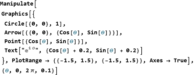
This interactive diagram shows how increasing the angle θ rotates the point around the unit circle exactly as ![]() predicts.
predicts.
Reflect on how Euler’s Formula turns multiplication of complex numbers into addition of angles. Euler’s Formula is a crown jewel of mathematics. It reveals that exponential functions and trigonometric functions are two sides of the same coin—a discovery that will profoundly influence everything.
Exercise 21.79: Consider (21.94)
1) Raise this complex number to the 4th power using Euler’s Formula. Simplify your answer and express it in rectangular form a+b i.
2) Verify your result by converting to polar form and using De Moivre’s Theorem.
Exercise 21.80: Consider (21.93)
1) In Wolfram Language, define ![]() and plot the points z(θ),z(2θ),z(3θ),z(4θ) on the complex plane for θ=π/12 (15°).
and plot the points z(θ),z(2θ),z(3θ),z(4θ) on the complex plane for θ=π/12 (15°).
2) Explain geometrically what multiplying by ![]() does to a complex number on the unit circle.
does to a complex number on the unit circle.
Hyperbolic Functions
When we combine exponential functions with the structure of trigonometry, an entirely new family of functions emerges that behaves in strikingly familiar yet different ways. These functions appear throughout physics—from the shape of hanging cables to special relativity and wave equations. Just as the trigonometric functions sine and cosine can be defined using the unit circle, we can define a parallel set of functions using the exponential function. These are called hyperbolic functions because their defining relations involve the hyperbola ![]() instead of the unit circle.
instead of the unit circle.
Definition 21.17 Definitions Using Exponentials: The two fundamental hyperbolic functions are defined directly in terms of the exponential function
![]()
(21.95)
and
![]()
(21.96)
From these we define the remaining hyperbolic functions by analogy with trigonometry
![]()
(21.97)
![]()
(21.98)
![]()
(21.99)
![]()
(21.100)
Hyperbolic functions mirror trigonometric functions in many ways, but with important sign differences:
| Trigonometric | Hyperbolic | Key Difference |
| Minus instead of plus. | ||
| sin (-x)=-sin x | sinh(-x)=-sinh x | Odd functions |
| cos (-x)-cos x | csh (-x)=-cosh x | Even functions |
| Addition fomrulas | Very similar addition formulas | Sign changes |
Examples of the addition formulas,
![]()
(21.101)
and
![]()
(21.102)
We can plot these functions.
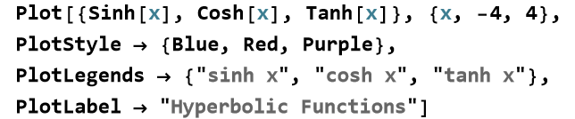
We can see that cosh x looks like a hanging chain (a catenary). We can see that sinh x is an odd function passing through the origin. And tanh x approaches + 1 as x → +∞ and − 1 as x → −∞.
Let’s say we want to solve
![]()
(21.103)
Using the definitions and the identity ![]() , or by expressing everything in exponentials, we find x=ln 2.
, or by expressing everything in exponentials, we find x=ln 2.
Let’ say we want to compute cosh(ln3),
![]()
(21.104)
Hyperbolic functions are not just mathematical curiosities—they are essential tools in relativity, electromagnetism, and classical mechanics. Mastering them gives you another powerful bridge between exponentials and geometry.
Exercise 21.81: Using the exponential definitions, compute the following by hand:
1) sinh(ln 2)
2) cosh(ln 3)
3) tanh (1)
Exercise 21.82: Prove the hyperbolic identity ![]() .
.
Exercise 21.83: Solve the following equations for x:
1) 5 sinh x = 3 cosh x
2) cosh x=2
3) tanh x = 0.8
Exercise 21.84: Explain the main similarities and differences between hyperbolic functions and trigonometric functions.
Summary
Write a summary for this lesson.
For Further Study
Jerrold E. Marsden, Alan Weinstein, (1985), Calculus I. Springer-Verlag, New York. You can download it for free from CalTech: https://www.cds.caltech.edu/~marsden/volume/Calculus/
What’s so special about Euler’s number e? (3Blue1Brown)
→ One of the best visual explanations of ( e ) and natural logs.
https://www.youtube.com/watch?v=m2MIpDrF7Es
What makes the natural log “natural”? (3Blue1Brown – Lockdown Live Math)
Deep, intuitive follow-up on why lnx\ln x\ln x
is special.
https://www.youtube.com/watch?v=4PDoT7jtxmw
Introduction to Logarithms (Eddie Woo) – Full series
Extremely clear and engaging for beginners.
https://www.youtube.com/watch?v=ntBWrcbAhaY (Part 1)
Playlist: https://www.youtube.com/playlist?list=PL5KkMZvBpo5D2djP07pTNWY3QnBqEASKf
Exponential & Logarithmic Functions (Professor Leonard) – Full College Algebra Playlist
Thorough, patient, and excellent for self-study.
https://www.youtube.com/playlist?list=PL-PeT1U2DANjhelvEy9YJe_-PdfSM2LR6
Solving Exponential and Logarithmic Equations (Professor Dave Explains)
Clear step-by-step solving techniques.
https://www.youtube.com/watch?v=10I_TVuYLkQ
Calculus I: Exponential and Logarithmic Functions (Math for Thought)
Good bridge from precalculus to calculus.
https://www.youtube.com/watch?v=Fhdn9CTUZOc
Hyperbolic Functions & Their Connection to Exponentials (Dr. Peyam)
Excellent for the hyperbolic section you’re writing.
Search “Dr. Peyam hyperbolic functions” (multiple great short videos)
Visualizing Exponentials and Logs (Numberphile / Mathologer)
Fun, high-quality motivational videos.
Example: Search “Numberphile e” or “Mathologer logarithms”