Lesson 20 Calculus 2 Differentiation in One Variable

“The tangent line is the best linear approximation to the curve at a point—and that idea is profound.” Gilbert Strang

“Differentiation is not just a mathematical operation—it is a way of seeing the instantaneous truth hidden in continuous change.” Henri Poincaré

Introduction

We began our study of calculus with limits and continuity—the mathematical language for describing how functions behave as we approach a point. Now we take the decisive next step by learning how to measure the instantaneous rate of change of a function. This is the heart of differential calculus. The derivative tells us how fast a quantity is changing at any given moment. It transforms our understanding from average rates (such as average velocity) to instantaneous rates (such as instantaneous velocity). It is the tool that lets us move from the static description of a system to its dynamic behavior. The process of finding derivatives is called differentiation, and that is the mathematics of “right now.” It answers the question, “At this precise instant, how rapidly is this quantity changing?”

In this lesson we will start with the rigorous epsilon-delta definition of the derivative. We will explore differentials, learn step-by-step methods for calculating derivatives, and study higher-order derivatives. You will see how velocity and acceleration are simply the first and second derivatives of position. We will examine real physical applications such as thermal expansion, and learn how to compute and visualize derivatives using Wolfram Language. We will investigate the deep relationship between differentiability and continuity, explore what it means for a function to be continuous but not differentiable, and prove important results such as the uniqueness of derivatives. Finally, we will master the basic rules of differentiation, the powerful Chain Rule, implicit differentiation, and the elegant Mean Value Theorem.

By the end of this lesson you will have the ability to find the instantaneous rate of change of almost any function, interpret derivatives physically, and use Wolfram Language to visualize how functions change. This is where calculus truly begins to reveal the dynamic nature of the physical world — from the motion of planets to the flow of heat to the behavior of electric circuits.You have worked hard to reach this point. The concepts in this lesson will reward your effort many times over as we continue our journey through calculus and theoretical physics.

Let us begin.

The Epsilon-Delta Definition of the Derivative

We have learned how to talk rigorously about limits using the epsilon-delta definition. Now we apply that same precision to the most important new idea in calculus: the derivative. The derivative tells us the instantaneous rate of change of a function at a particular point — how fast the output is changing exactly at that moment. The derivative at a point a is the number that best describes how the function behaves in an arbitrarily small neighborhood around a. It is the slope of the best linear approximation to the curve at that point. Just as we used epsilon and delta to define what it means for a function to approach a value, we now use them to define the instantaneous rate of change.

Definition 20.1 The Epsilon-Delta Definition of the Derivative: A function f is said to be differentiable at x=a, and its derivative at a is the value f'(a), if

(20.1)

which, in epsilon-delta language, means that for every ε>0, there exists a δ>0 such that if 0<∣h∣<δ, then

(20.2)

In plain language, “No matter how small an error tolerance ε you choose for the slope, you can always find a small enough interval around a (controlled by δ) such that the average rate of change (the slope of the secant line) stays within that tolerance of the true instantaneous rate f'(a).”

Imagine zooming in closer and closer to the point (a, f(a)) on the graph of f. The derivative f'(a) is the slope of the straight line that the curve looks more and more like as we zoom in. The epsilon-delta definition guarantees that we can make the secant lines (formed by points very close to a) have slopes as close as we want to this limiting tangent slope.

This rigorous definition ensures that our notion of “instantaneous rate of change” is not vague or hand-wavy—it is built on the same solid foundation as the rest of calculus.

The epsilon-delta definition of the derivative is the cornerstone of differential calculus. As we shall see later, it allows us to prove all the differentiation rules with complete certainty. While we will rarely use the full definition to compute derivatives in practice (we will use the powerful rules instead), understanding it gives you confidence that everything built upon it is trustworthy.

In the sections ahead, we will learn practical techniques for calculating derivatives and explore their many applications in physics — from velocity and acceleration to thermal expansion and beyond.

Exercise 20.1: Begin with Definition 20.1 and copy it into your notebook. Reflect on its meaning for a few minutes. Note any thoughts that come to mind. How would you explain this to someone sitting in front of you. Write this down.

Exercise 20.2:
a) Evaluate the following derivatives
    1)
    2)
    3)
b) State the epsilon-delta definition of the derivative of f at x=a in your own words.  Then explain what the symbols ε and δ represent mathematically in this context.
c) Consider the function f(x)=2x+3.  Use the epsilon-delta definition to prove that f'(3)=2. (Show the logical steps: start with “Let ε>0\epsilon > 0\epsilon > 0
    be given,” choose a suitable δ, and verify the inequality.)
d) Draw a sketch (or describe in words) of what the epsilon-delta definition means geometrically for the derivative at a point.  Include:The point (a, f(a)), a small horizontal band of width         2ε around the tangent line value, a corresponding vertical band of width 2δ around x=a. Explain what the definition guarantees about the secant lines in that region.
e) Why is the epsilon-delta definition of the derivative important, even though we will usually use simpler rules to compute derivatives?
f) How does this definition connect to the idea of the derivative as the slope of the tangent line?

Differentials and Derivatives

We have learned that the derivative f'(a) tells us the instantaneous rate of change of a function at a point. Now we introduce a closely related and very practical idea, differentials. Differentials give us a way to talk about small changes in both the input and the output of a function. If we make a very small change dx in the input x, the corresponding small change df in the output can be approximated using the derivative. The differential df is the linear approximation to the actual change Δ f when the input changes by a small amount dx.

Definition 20.2 Differentials: Let y=f(x). The differential of y (denoted dy) is defined as

(20.3)

Here dx is an arbitrary small change in the input x (sometimes called the increment, as we saw in Lesson 16), dy is the corresponding approximate change in the output, calculated using the derivative.

Geometrically, dy represents the vertical change along the tangent line when x changes by dx. The actual change in the function, Δ y=f(x+dx)−f(x), is usually very close to dy when dx is small.

This linear approximation is one of the most useful ideas in applied mathematics and physics.

Suppose we have y = . Then y'=2 x, so according to (20.3) we have dy=2 x dx. If x=3 and we make a small change dx=0.1, the approximate change in y is dy=2⋅3⋅0.1=0.6. The actual change is , which is very close to our estimate.

Differentials are extremely useful for estimating small changes and errors. For example,

How much does the volume of a sphere change if the radius increases by a tiny amount?

How much error in calculated area results from a small measurement error in length?

How does a small change in temperature affect the length of a metal rod (thermal expansion)?

In all these cases, differentials provide a quick and often sufficiently accurate linear approximation.

Differentials bridge the gap between derivatives (instantaneous rates) and practical estimation of small changes. They are a powerful tool you will use again and again in theoretical physics, engineering, and error analysis.

One notational due to (20.3) is

(20.4)

another way of writing the derivative as the ratio of the differentials.

Exercise 20.3: Begin with Definition 20.2 and copy it into your notebook. Reflect on its meaning for a few minutes. Note any thoughts that come to mind. How would you explain this to someone sitting in front of you. Write this down.

Exercise 20.4:
a) Let .
    1) Find the differential dy.
    2) If x=2 and dx=0.1, compute dy.
    3) Calculate the actual change Δ y=f(2.1)−f(2) and compare it with dy.
b) Consider the function at x=4.
    1) Find the differential dy.
    2) Use differentials to approximate .
    3)  Compare your approximation with the actual value and explain the accuracy.
c) The side of a square is measured to be 10 cm with a possible error of ±0.1 cm.
    1) Use differentials to estimate the maximum error in the calculated area.
    2) What is the relative error (as a percentage)?
    3) Explain why differentials are useful for error analysis.
d) The linear expansion of a metal rod is given by , where α is the coefficient of linear expansion.
    1) Express this using differentials.
    2) A steel rod has length m and . Use differentials to estimate the change in length when the temperature increases by 30°C.
    3) Discuss when this approximation is valid.
e) Explain in your own words the difference between the actual change and the differential.
f) Why is the differential (2.3) sometimes called the linear approximation?

Visualizing Derivatives

We have now defined the derivative rigorously using the epsilon-delta definition. While the formal definition gives us precision, seeing derivatives in action brings them to life. Visualization helps us develop strong intuition about what the derivative really represents: the slope of the tangent line at a point, the instantaneous rate of change, and the best linear approximation to the function near that point. A graph of a function together with its tangent line at a point makes the meaning of the derivative immediately clear. By watching secant lines approach the tangent line as the points get closer, we can literally see the limit definition in action. Visualization turns the abstract concept of the derivative into something we can see and feel.

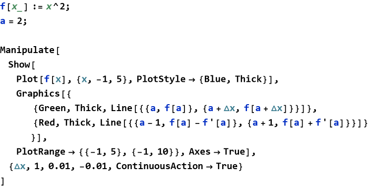
TAt any point where the derivative exists, the tangent line is the straight line that best matches the curve at that instant. Here is how we can visualize it in Wolfram Language.

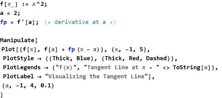
As you move the point a, watch how the red dashed tangent line touches the blue curve and matches its slope perfectly at that point.

We can also animate the process of the limit definition by showing secant lines getting closer to the tangent.

This visualization dramatically shows how the secant line slope approaches the tangent slope as Δ x gets smaller.

Visualizing derivatives is one of the most effective ways to move from formal understanding to deep physical insight. As we continue, this visual foundation will make the rules of differentiation and their applications in physics much more meaningful.

Differentiability and Continuity

We have now defined both continuity and the derivative using rigorous limit concepts. It is natural to ask, what is the relationship between these two important ideas? If a function is continuous at a point, does that mean it must be differentiable there? And conversely, if a function is differentiable, must it be continuous? Differentiability is a stronger condition than continuity. Every differentiable function is continuous, but not every continuous function is differentiable. Continuity means the function has no breaks or jumps. Differentiability means the function is smooth enough to have a well-defined tangent line at that point—it has an instantaneous rate of change.

Definition 20.3 Differentiability at a Point: A function f is said to be differentiable at x=a if the derivative f'(x) exists. That is, if the following limit exists

(20.5)

If a function f is differentiable at x=a, then f is continuous at x=a.

Theorem 20.1: If a function f is differentiable at x=a, then f is continuous at x=a.

Proof of Theorem 20.1: This is a direct proof. Since f is differentiable at a, the limit (20.5) exists. We need to show that f is continuous at a, that is

(20.6)

Let Δ x=x−a. As x→a, we have Δ x→0. Then

(20.7)

Taking the limit as x→a (i.e., as Δ x→0)

(20.8)

Because the limit of a sum is the sum of the limits (provided they exist), this becomes

(20.9)

We know the first limit is f'(a) by differentiability, and the second limit is 0. Therefore

(20.10)

This shows that f is continuous at x=a. QED

If the derivative exists, the function must be “smooth enough” at that point for the tangent line to make sense. A function with a sharp corner or a jump cannot have a well-defined tangent slope, so it cannot be differentiable. However, a function can be continuous (no jumps or breaks) but still have corners or cusps where the tangent line is not well-defined.

For example we can examine the absolute value function

(20.11)

This function is continuous everywhere, including at x=0. However, it is not differentiable at x=0 because the left-hand and right-hand derivatives differ (the graph has a sharp corner).

As another example, some functions are continuous but have a sharp point (cusp) where the slope becomes infinite or undefined from one side.

In physics, we often assume functions are differentiable because we want well-defined rates of change. However, real systems sometimes have points where this assumption breaks down—for example, at the moment of impact, at phase transitions, or at boundaries between different materials. Recognizing where a function is continuous but not differentiable helps us understand the limitations of our models.

Understanding the relationship between differentiability and continuity gives you a more refined view of how functions behave. It prepares you to recognize when our calculus tools apply smoothly and when we must be more careful.

Exercise 20.5: Begin with Definition 20.3 and copy it into your notebook. Reflect on its meaning for a few minutes. Note any thoughts that come to mind. How would you explain this to someone sitting in front of you. Write this down. Do this for the definition, theorem, and proof.

Step-by-Step Evaluation of Derivatives

We now understand what the derivative means both conceptually and rigorously. The next practical skill is learning how to compute derivatives efficiently and confidently. While the epsilon-delta definition provides the foundation, we can usually evaluate derivatives by following a clear, repeatable process of simplification and careful calculation. Computing a derivative is not mysterious. It is a systematic procedure of rewriting the expression, applying limit techniques where needed, and simplifying the result. A step-by-step method turns differentiation into a reliable skill rather than a guessing game.

To find the derivative of a function f(x), follow these steps:

Step 1: Write down the definition of the derivative (when helpful for understanding)

(20.12)

Note that we can use the prime notation f'(x) or the notation due to the German polymath Gottfried Wilhelm Leibniz (1646-1716), the coinventor with Sir Isaac Newton of calculus, dy/dx. These options may be used interchangeably.

Step 2: Simplify the expression inside the limit.

Step 3: Evaluate the limit.

Step 4: Interpret the result.

Step 5: Verify (optional but recommended).

As a first example we have a simple polynomial. Let

(20.13)

Write the difference quotient that we met in Lesson 16

(20.14)

Expand and simplify

(20.15)

Take the limit as Δ x→0

(20.16)

For a second example we look at a rational function,

(20.17)

First simplify the function

(20.18)

Then apply the difference quotient to the simplified form and take the limit to get

(20.19)

As a third example, we examine a square root function

(20.20)

We find the difference quotient

(20.21)

Rationalize the numerator

(20.22)

Take the limit as Δ x→0

(20.23)

By following this step-by-step approach consistently, you build both skill and confidence. As we learn more techniques in the coming sections, this systematic process will become faster and more automatic. The goal is not just to get the right answer, but to understand why each step works. Mastering this methodical approach to evaluating derivatives is a foundational skill that will serve you throughout calculus and theoretical physics.

Exercise 20.6:
a) Let .
    1) Write the difference quotient.
    2) Simplify the expression algebraically.
    3) Take the limit as Δ x->0 to find the derivative.
b) Let .
    1) Simplify the function.
    2) Write the difference quotient.
    3) Take the limit as Δ x->0 to find the derivative.
c) Let
    1) Write the difference quotient.
    2) Rationalize the  numerator.
    3) Take the limit as Δ x->0 to find the derivative.
d) Let .
    1) Use the step-by-step method to find the general derivative.
    2) Evaluate the derivative at x=2
    3)  Interpret the result as the slope of the tangent line at that point.
e) Let .
    1)  Simplify the function first, then find the derivative using the step-by-step method.
    2) Compare this with what happens if you try to plug in x=−3 directly into the original expression.
    3) Explain why simplification is often necessary.
f) Why is it useful to follow a systematic step-by-step procedure when evaluating derivatives?
g) In which situations is algebraic simplification of the difference quotient most helpful?
h) How does this methodical approach help build confidence when working with more complicated functions?

The Binomial Theorem

As we compute derivatives using the definition, we encounter expressions like . Expanding these by hand for higher powers would be tedious. Fortunately, there is a powerful and elegant theorem that does this work for us systematically. When you raise a binomial (a sum of two terms) to a positive integer power, you can expand it using a predictable pattern of coefficients.

Theorem 20.2 The Binomial Theorem: For any positive integer n,

(20.24)

where we can write the binomial coefficient

(20.25)

So we can write ,

(20.26)

In expanded form, this becomes

(20.27)

Proof of Theorem 20.2: This is a proof by mathematical induction. We begin with the base case (n=1)

(20.28)

This holds true for the base case.

Inductive Hypothesis: Assume the theorem is true for some positive integer k

(20.29)

Inductive Step (prove for n=k+1)

We need to show that

(20.30)

Start with the left side

(20.31)

By the inductive hypothesis,

(20.32)

We apply distribution

(20.33)

Shift the index in the second sum by letting j=m+1

(20.34)

Combine like terms. For the term we have m=0, so

(20.35)

For the term where j=k+1 we have

(20.36)

For the middle terms where 1≤m≤k

(20.37)

(You can verify this identity using the definition of binomial coefficients.)

Thus,

(20.38)

This completes the inductive step.

So, by the principle of mathematical induction, the Binomial Theorem holds for all positive integers n. QED

For example, we need to expand

(20.39)

Example 2: Expand

(20.40)

Basic Rules of Differentiation

We now understand what the derivative means and how to evaluate it using the definition when necessary. Fortunately, most derivatives can be computed much more efficiently using a small set of powerful rules. These rules, which follow logically from the limit properties we proved earlier, allow us to differentiate complicated functions quickly and confidently. Differentiation is linear and follows predictable patterns. Once you know these basic rules, you can break down almost any function into simpler pieces and differentiate term by term. The rules of differentiation turn a difficult limit problem into a straightforward algebraic procedure.

Theorem 20.3 The Constant Rule: The derivative of a constant is zero. f(x)=c⇒f'(x)=0.
For example, the derivative of 7 is 0, since 7 does not change.

Exercise 20.7: Prove Theorem 20.3.

Theorem 20.4 Power Rule: For any real number n

(20.41)

For example, .

Proof for Theorem 20.4: This is a direct proof. Let . By definition

(20.42)

Step 1: Expand using the Binomial Theorem.

(20.43)

So, we subtract by

(20.44)

Step 2: Divide by Δ x

(20.45)

Step 3: Take the limit as Δ x->0. As Δ x approaches 0, every term containing Δ x (or higher powers) goes to zero. Therefore,

(20.46)

Thus

(20.47)

QED

Theorem 20.5. Constant Multiple Rule:

(20.48)

Exercise 20.8: Prove Theorem 20.5.

Theorem 20.6 Sum and Difference Rule:

(20.49)

(20.50)

Proof of Theorem 20.6: This is a direct proof. By definition of the derivative,

(20.51)

Step 1: Rewrite the difference quotient

(20.52)

Step 2: Split the limit, using the limit law for sums,

(20.53)

Step 3: Apply the definition of the derivative, where the first limit is exactly f'(x), and the second limit is exactly g'(x). Therefore, (20.49) holds true.

For the Difference Rule, simply replace +g(x) with −g(x). The same steps apply, yielding (20.50).

Theorem 20.7 Product Rule:

(20.54)

Proof of Theorem 20.7: This is a direct proof. By definition of the derivative,

(20.55)

Step 1: We add and subtract f(x+Δ x)g(x) inside the numerator

(20.56)

Step 2: Group the terms

(20.57)

Step 3: We can now split the limit (using the sum and product rules for limits

(20.58)

Step 4: Substituting the known limits

(20.59)

QED

Theorem 20.8. Quotient Rule:

(20.60)

Exercise 20.9: Prove Theorem 20.8.

You now have the ability to compute the instantaneous rate of change for a wide variety of functions — a skill that will serve as the foundation for the rest of calculus and its many applications in theoretical physics.

Exercise 20.10: Begin with Theorem 20.3 and copy it into your notebook. Reflect on its meaning for a few minutes. Note any thoughts that come to mind. How would you explain this to someone sitting in front of you. Write this down. Do this for each theorem, and proof.

Exercise 20.11:
a) Differentiate the following functions:
    1) f(x)=7
    2)  


    3)
b) Find the derivative:
    1)
    2)
c) Differentiate the following functions:
    1)
    2)
d) Differentiate:
    1)
    2)
e) Find the derivative:
    1)
    2)
f) Explain in your own words why the Product Rule and Quotient Rule are necessary.
g) Give an example of a function where you would need to use the Product Rule.
h)  Why is it important to master these basic rules?

Trigonometric Derivatives

We have learned the basic rules for differentiating polynomials, products, and quotients. Now we turn to one of the most beautiful and useful families of functions in physics, the trigonometric functions. Derivatives of sine, cosine, and tangent appear frequently—from the motion of pendulums and springs to wave phenomena and alternating current circuits. The derivatives of sine and cosine are simple cyclic shifts of the original functions. This elegant relationship is one of the reasons trigonometry is so powerful in modeling periodic phenomena. Differentiating trigonometric functions reveals deep connections between rates of change and the original functions themselves.

Theorem 20.9:

(20.61)

Proof of Theorem 20.9: This is a direct proof. By definition,

(20.62)

Step 1: Use the sine addition formula

(20.63)

so

(20.64)

Therefore,

(20.65)

Step 2: Take the limit as Δ x->0

(20.66)

Step 3: Evaluate the two known limits. We already know from previous work that

(20.67)

For the other limit, we use the identity

(20.68)

Step 4: Combine the results

(20.69)

QED

Theorem 20.10:

(20.70)

Proof of Theorem 20.10: This is a direct proof. By definition,

(20.71)

Step 1: Use the cosine addition formula

(20.72)

so

(20.73)

Therefore,

(20.74)

Step 2: Take the limit as Δ x->0

(20.75)

Step 3: Evaluate the two known limits. We already know

(20.76)

For the other limit, using the identity

(20.77)

Step 4: Combine the results

(20.78)

QED

Theorem 20.11:

(20.79)

Proof of Theorem 20.11: This is a direct proof. We know that

(20.80)

Let f(x)=sin⁡ x and g(x)=cos⁡ x.

By the Quotient Rule,

(20.81)

We already proved that f'(x)=cos x and g'(x)=-sin x.

Substituting these in

(20.82)

By the Pythagorean identity

(20.83)

QED

For example

(20.84)

We begin by using the product rule,

(20.85)

For another example

(20.86)

By the quotient rule,

(20.87)

Mastering trigonometric derivatives opens the door to analyzing oscillatory motion, waves, and many other periodic phenomena in physics. As we continue, you will see these derivatives appear again and again — they are among the most frequently used tools in theoretical physics.

Exercise 20.12: Begin with Theorem 20.9 and copy it into your notebook. Reflect on its meaning for a few minutes. Note any thoughts that come to mind. How would you explain this to someone sitting in front of you. Write this down. Do this for each theorem, and proof.

Exercise 20.13:
a) Differentiate the following functions:
    1) f(x)=sin (5 x)
    2)  f(x)=3 cos (2x)


    3) f(x)=tan (4x)
b) Find the derivative:
    1)
    2)
    3) f(x)=sin x cos 2 x
c) Differentiate the following functions:
    1)
    2) f(x)=(sin x)/(1 + cos x)
    3) f(x)=x tan 3 x
d) Differentiate:
    1)
    2)
e) Find the derivative:
    1)
    2)

Higher-Order Derivatives

We have learned how to find the derivative of a function—the instantaneous rate of change. Many phenomena in physics, however, require us to look deeper. We often need to know how fast that rate of change itself is changing. This leads us to the powerful idea of higher-order derivatives. We can differentiate a function repeatedly. Each new derivative tells us something important about the behavior of the original function. The second derivative tells us the rate of change of the first derivative (concavity or acceleration). The third derivative tells us the rate of change of the second derivative, and so on.

Definition 20.4 Higher-Order Derivative: The nth derivative of a function, denoted , is the derivative of . The second derivative can also be denoted f''(x) or

(20.88)

The third derivative is denoted f'''(x) or

(20.89)

For example, in the case of a polynomial, let

(20.90)

The first derivative is

(20.91)

The second derivative is

(20.92)

The third derivative is

(20.93)

The fourth derivative is

(20.94)

The fifth derivative and higher is just 0.

In another example we choose the trigonometric function

(20.95)

The first derivative is

(20.96)

The second derivative is

(20.97)

The third derivative is

(20.98)

The fourth derivative is

(20.98)

Notice the beautiful cycle of length 4.

Higher-order derivatives give us a much richer picture of how a function behaves. They are essential tools for understanding motion, wave behavior, electric circuits, and many other systems in theoretical physics.

Exercise 20.14: Begin with Definition 20.4 and copy it into your notebook. Reflect on its meaning for a few minutes. Note any thoughts that come to mind. How would you explain this to someone sitting in front of you. Write this down.

Exercise 20.15:
a) For .
    1) Find the first derivative.
    2) Find the second derivative.


    3) Find the third derivative
    4) Find the fourth derivative.
b) For g(x)=sin 2 x+3 cos 4 x.
    1) Compute the first four derivatives.
    2) Describe the pattern you observe.
    3) Predict what will be without computing all steps.
c) Explain in your own words what the second derivative tells us about the graph of a function.

Differentiation in the WL

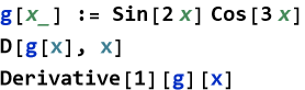
We have now learned how to compute derivatives by hand using rules and definitions. Wolfram Language (WL) makes this process effortless while giving us powerful tools for symbolic, numerical, and visual exploration. Mastering differentiation commands in WL will save you time and let you focus on understanding the physics rather than tedious algebra. WL provides two main ways to differentiate — the D[] command for direct computation and the Derivative[] operator for creating derivative functions that you can apply repeatedly or to pure functions. In WL, differentiation becomes a natural, symbolic operation that mirrors the mathematical rules we have been studying.

The D[] command allows you to calculate derivatives. Here is the syntax:

For example, note that if we define a function f[x], the derivative is f’[x].

As another example, we take a second derivative.

The more elegant and powerful tool is Derivative[n], which creates a pure derivative function.

We define

So,

We get the same thing.

Here is the second derivative.

Then a third derivative.

This is especially useful when you want to define a new function that is the derivative.

Here is another trigonometric function.

Here we have higher-order derivatives.

Here is why Derivative[] is powerful:

It creates reusable derivative functions.

It works beautifully with pure functions.

It makes higher - order derivatives clean and readable.

It works perfectly with Plot, Manipulate, and Solve.

Suggested Activity: Define a position function in WL. Use both D[] and Derivative[] to find the first three derivatives. Then create an interactive Manipulate plot showing all of them together. Observe how the zeros of velocity correspond to turning points in position, and how the sign of acceleration relates to concavity.

Mastering differentiation in Wolfram Language transforms you from someone who computes derivatives into someone who explores them . You can now instantly move from symbolic expressions to graphs, numerical values, and physical insight — a skill that will serve you throughout the rest of this book and in all your future work in theoretical physics.

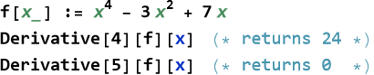
Exercise 20.16:
a) Define in Wolfram Language.
    1) Use D[f[x], x] to compute the first derivative.
    2) Use Derivative[1][f][x] to compute the same derivative.


    3) Use Derivative[2][f][x] to find the second derivative.
    4) Compare the outputs and explain any differences in form.
b) For .
    1) Compute the first through fourth derivatives using both D[] and Derivative[].
    2) Use Derivative[5][g][x] and explain the result.
    3) What pattern do you observe in the higher-order derivatives of polynomials?
c) Define h(x)=sin⁡(3x)cos⁡(2x).
    1) Compute h’[x] using D[].
    2) Compute the second derivative h’’(x) using Derivative[2][h].
    3) Simplify the result by hand using trigonometric identities and compare with WL’s output.
d) Define .
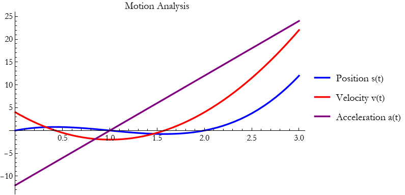
    1) Create a single Plot showing f[x], f’[x], and f’’[x] together with distinct colors and a legend.
    2) Use Manipulate to let the user vary a point a and display the value of f’’[a].
    3) Describe the geometric relationship between the sign of f’’[x] and the shape of f[x].
e) Explain the advantage of using Derivative[n][f] over repeatedly applying D[].
f) In what situations would you prefer one method over the other?

Velocity and Acceleration as Derivatives

We have now developed the mathematical machinery of differentiation. It is time to see one of its most direct and powerful applications in physics, the ability to describe the motion of objects. The first and second derivatives of position with respect to time give us velocity and acceleration—two of the most important quantities in classical mechanics. Derivatives turn a description of where an object is into a description of how it is moving. Position is a function of time. Its first derivative is velocity (how fast and in what direction it is moving). Its second derivative is acceleration (how quickly the velocity is changing).

If we label the position function as s(t), then velocity is

(20.100)

Acceleration is then

(20.101)

For example, a particle moves according to

(20.102)

Then the velocity is,

(20.103)

The acceleration is then,

(20.104)

At t=1 sec, s(t)=0 m, v(t)=-2 m , and a(t)=0 m . From this we see that there is no acceleration, so velocity is constant.

Let’s say we have a mass on a spring with position s(t)=0.3sin⁡(4π t) m. Then the velocity is v(t)=0.3⋅4 πcos⁡(4π t)=1.2π cos⁡(4π t) m . The resulting acceleration is a(t)=−1.2π 4πsin⁡(4π t)=−4.8π 2sin⁡(4π t) m . Notice that acceleration is proportional to −sin⁡(4π t), which is −s(t). This is the hallmark of simple harmonic motion.

In Wolfram Language we can write,

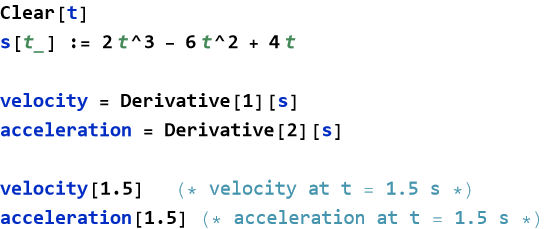
Positive velocity ⇒ moving in the positive direction  
Negative velocity ⇒ moving in the negative direction  
Positive acceleration ⇒ speeding up (in the positive direction) or slowing down (if moving negative)  
When velocity and acceleration have the same sign, the object is speeding up.  
When they have opposite signs, the object is slowing down.

Understanding velocity and acceleration as derivatives is a major milestone. You can now move fluidly between position, velocity, and acceleration—the foundation of kinematics and a key tool you will use throughout classical mechanics, electromagnetism, and beyond.

As a note, you can take higher derivatives of position. The third derivative is called jerk, and is important in engineering. A high jerk is uncomfortable for passengers, so engineers try to minimize this for comfort. The fourth derivative is called snap or jounce. The fifth derivative derivative is called crackle. The sixth derivative is called pop. These are used in robotics, spacecraft control vibration analysis, and any time extremely smooth motion is required.

Exercise 20.17:
a) Define in Wolfram Language.
    1) Find the velocity.
    2) Find the acceleration.


    3) Evaluate velocity and acceleration at t=2 seconds.
    4) Find the times when the particle is at rest (v(t)=0).
    5) Determine the intervals where the particle is speeding up and slowing down.
    6) Interpret the physical motion of the particle.
c) A mass on a spring has position s(t)=0.25sin⁡(8π t) meters.
    1) Find the velocity and acceleration.
    2) Examine the acceleration. How does it relate to position?
    3)  What does this relationship tell you about the motion?
d) Define in WL.
    1) Use Derivative[] to define velocity and acceleration functions.
    2) Compute velocity and acceleration at t=1.5 sec.
    3) Create a Plot showing position, velocity, and acceleration on the same graph (use different colors and a legend).
e) The velocity of a car is m/sec.
    1) Find the acceleration function.
    2) At what time(s) is the car at rest?
    3) When is the car speeding up? When is it slowing down?
    4) Describe the motion in everyday language.
f) The position function is .
    1) Find the velocity.
    2) Find the acceleration.
    3) Evaluate acceleration at t=π/4.
g) Consider the idea of the graphs of position, velocity, and acceleration.
    1) Explain what a positive second derivative means geometrically on the position graph.
    2) If velocity is positive and acceleration is negative, what is happening to the particle’s speed?
    3) Sketch a possible position graph consistent with v(t)>0 and a(t)<0 for 0<t<2.
h) Why is acceleration the derivative of velocity rather than just “change in velocity over time”?
i) Give a real-world example (other than a car or spring) where knowing the second derivative is physically important.
j) Explain the relationship between the zeros of velocity and turning points in position.

The Chain Rule

We now know how to differentiate polynomials, products, quotients, and trigonometric functions. Many functions in physics, however, are composed—one function placed inside another. The position of a moving object might depend on velocity, which itself depends on time in a complicated way. To handle these situations we need one of the most powerful tools in calculus, the Chain Rule. When a function is composed of an “outer” function applied to an “inner” function, the derivative is the derivative of the outer function (evaluated at the inner function) multiplied by the derivative of the inner function. The rate of change of the whole is the rate of change of the outer part times the rate of change of the inner part.

Theorem 20.12 The Chain Rule:

Let y=f(g(x)), where f is the outer function and g is the inner function. If both f and g are differentiable, then

(20.105)

where u=g(x). In prime notation

(20.106)

Proof of Theorem 20.12: This is a direct proof. Let u=g(x). We must show

(20.107)

Define the difference quotient for f. For k≠0, let

(20.108)

By the definition of f'(u), we have . We can also define φ(0)=0 so that φ is continuous at 0.

Now write the difference quotient for the composite function

(20.109)

where Δ x=g(x + Δ x - g(x)).

If Δ x≠0, then

(20.110)

If Δ x=0, then the left side is 0, and the right side is also 0 (since Δ u/Δ x=0).

So in all cases we can write

(20.111)

Now take the limit as Δ x→0. Since g is differentiable (hence continuous), Δ u→0 as Δ x→0. Therefore φ(Δ u)→φ(0)=0.Thus,

(20.112)

QED

Imagine a machine with two gears. The inner gear turns at rate g'(x). The outer gear turns at rate f'(u) when its input is u. The overall speed of the output is the product of the two rates.

For example, let .

We can write the inner function,

(20.113)

Then the outer function is,

(20.114)

By the Chain Rule

(20.115)

For the trigonometric function,

(20.116)

We have the inner function,

(20.117)

The outer function is,

(20.118)

The Chain Rule gives us the result

(20.119)

For a physics example, suppose the radius of a raindrop increases as it falls

(20.120)

The volume is,

(20.121)

So,

(20.122)

Then

(20.123)

Substituting gives the rate at which the volume (and therefore mass) is increasing.

(20.124)

Here is an example from Wolfram Language.

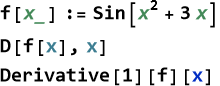
Both commands return the same result using the Chain Rule internally.

The Chain Rule lets us differentiate extremely complicated functions by breaking them into simpler pieces. Almost every real physical system involves some form of composition: position depends on velocity, velocity depends on force, force depends on position, and so on. Mastering the Chain Rule is therefore essential for theoretical physics.

Suggested Activity: Choose three composite functions of increasing difficulty (e.g., {, ,Tan[Cos[2 x]]}). Differentiate each by hand using the Chain Rule. Then verify your answers in Wolfram Language. Create a small table showing the outer function, inner function, and the two derivatives you multiplied.

The Chain Rule is one of the great unifying ideas of calculus. Once you become comfortable with it, you will be able to tackle almost any derivative that appears in physics—from planetary motion to electrical circuits.

Exercise 20.18: Begin with Theorem 20.12 and copy it into your notebook. Reflect on its meaning for a few minutes. Note any thoughts that come to mind. How would you explain this to someone sitting in front of you. Write this down. Also do this for the proof.

Exercise 20.19:
a) Differentiate using the Chain Rule
    1)


    2)


    3)
c) Find the derivative
    1)
    2)
    3)  
d) Differentiate:
    1)
    2) .
    3) f(x)=cos (sin(3x))
e) The position of a particle is meters.
    1) Find the velocity.
    2) Find the acceleration.
    3) Evaluate the velocity and acceleration at t=1 second.
f) Define f(x)=sin⁡(x2)cos⁡(3x) in Wolfram Language.
    1) Compute the first derivative using D[].
    2) Compute the first derivative using Derivative.
    3) Create a plot of f(x) and f'(x) together. What is the relationship the plot shows?
g) Explain in your own words why the Chain Rule is necessary when dealing with composite functions.
h) Give a real-world physical situation (other than the one in Exercise e) where a composite function naturally appears and the Chain Rule is required.

Implicit Differentiation

So far we have differentiated functions that are given explicitly—that is, where y is written directly as a function of x, such as . In physics and geometry, however, relationships between variables are often given implicitly—as an equation involving both x and y without solving for one in terms of the other. Examples include circles, ellipses, and many physical laws. For these situations we need a powerful technique called implicit differentiation. Even when y is not isolated, we can still find dy/dx by differentiating both sides of the equation with respect to x, treating y as a function of x, and then solving for the derivative. Differentiate the entire equation as it stands, remembering that y depends on x, so every time you differentiate y you must multiply by dy/dx  (the Chain Rule in action).

Algorithm 20.1 The Method of Implicit Differentiation: Given an equation F(x,y)=0

Differentiate both sides with respect to x.

Apply the Chain Rule to any term containing y, d/dx g(y)=g'(y)(dy/dx).

Collect all terms containing dy/dx on one side.

Solve for dy/dx.

Consider the unit circle

(20.125)

Differentiate both sides with respect to x

(20.126)

Solve for the derivative:dy/dx.

(20.127)

This gives the slope of the tangent line at any point (x, y) on the circle (except where y=0).

We now turn to the the ellipse

(20.128)

Differentiate implicitly

(20.129)

A ladder 5 meters long leans against a wall. The base is pulled away from the wall at 0.2 m/s. How fast is the top sliding down when the base is 3 meters from the wall?

Let x = distance from wall to base, y = height of the top. Then

(20.130)

We then differentiate with respect to time t

(20.131)

When x=3 meters, y=4 meters, and dx/dt=0.2 m/sec

(20.132)

So, the top is sliding down at 0.15 m/sec.

Wolfram Language handles implicit differentiation naturally.

WL can solve for ( y'(x) ) automatically.

Many important curves and physical relationships cannot be easily solved for one variable. Implicit differentiation lets us find slopes, velocities, and rates of change without algebraic rearrangement. It is essential in related-rates problems, orthogonal trajectories, and advanced physics.

Mastering implicit differentiation greatly expands the kinds of problems you can solve. You are now equipped to handle equations that describe circles, ellipses, hyperbolas, and many real physical situations where variables are intertwined.

Exercise 20.20:
a) For each equation, find dy/dx:
    1)


    2)


    3)
b) Consider the curve defined by .
    1) Find dy/dx.
    2) Evaluate the slope at (1,1)
    3) Write the equation of the tangent line at (1,1).
c) Differentiate:
    1)
    2) .
d) A spherical balloon is being inflated so that its volume increases at a constant rate of 8 /sec.
    1) Write the relationship between volume and radius..
    2) Use implicit differentiation with respect to time to find dV/dt.
    3) How fast is the radius changing at 5 seconds.
e) Consider the equation .
    1) Compute y'(x).
    2) Evaluate the derivative at the point (1, 1).
    3) Plot the curve and the tangent line at (1, 1) using the result.
f)  Explain when you should use implicit differentiation instead of solving for y explicitly.
g) Why does the Chain Rule appear naturally in implicit differentiation?
h) Give a physical or geometric situation (other than the balloon problem) where implicit differentiation and related rates are useful. Describe the variables and the relationship.

The Mean Value Theorem

We have learned how derivatives describe instantaneous rates of change. Now we ask a deeper question, “What can the derivative tell us about the average rate of change of a function over an interval?” The answer is given by one of the most elegant and useful results in all of calculus—the Mean Value Theorem. This theorem connects the average slope of a function to its instantaneous slope at some point inside the interval. If a function is continuous on a closed interval and differentiable inside it, then there must be at least one point where the instantaneous rate of change equals the average rate of change over the whole interval. The tangent line at some point inside the interval is parallel to the secant line connecting the endpoints.

Before stating the full theorem, we first look at a simpler but extremely important special case.

Theorem 20.13 Rolle’s Theorem: Let f be continuous on the closed interval [a, b] and differentiable on the open interval (a, b). If f(a)=f(b), then there exists at least one number c in (a, b) such that

(20.133)

What does this actually mean? If the function starts and ends at the same height, and is smooth enough to have a tangent everywhere inside, then somewhere in between the tangent must be perfectly horizontal—the instantaneous slope is zero.

Because the function is continuous, it must reach a highest point and a lowest point somewhere in [a, b]. At any interior highest or lowest point, the tangent line (if it exists) must be horizontal. Therefore, there is at least one point where (20.133) holds.

Proof of Theorem 20.13: This is a direct proof by cases. Because f is continuous on the closed, bounded interval [a, b], it must attain both a maximum value and a minimum value somewhere in the interval (this is a fundamental property of continuous functions on closed intervals). There are three possible cases:

Case 1: The maximum or minimum occurs at an interior point c where a<c<b. At this interior extreme point, the tangent line (if it exists) must be horizontal (otherwise the function could go higher or lower nearby). Since f is differentiable at c, we have (20.133). This gives the desired point.

Case 2: The maximum and minimum both occur only at the endpoints. Since f(a)=f(b), the function is constant on [a, b] (it reaches the same value at both ends and never goes higher or lower). For a constant function, the derivative is zero  everywhere in (a, b). So any c works.

Case 3: One extreme is at an endpoint and the other is interior. The interior extreme again gives (20.133).

In all cases, there exists at least one c in (a, b) where (20.133) holds. QED

Theorem 20.14 Mean Value Theorem: Let f be continuous on [a, b] and differentiable on (a, b). Then there exists at least one number c in (a, b) such that

(20.134)

Here the instantaneous rate of change at some interior point equals the average rate of change over the entire interval.

Definition 20.5 Auxiliary Function: An auxiliary function is a new function, built from the original functions of some problem, that is designed to simplify the proof or solution. It usually has convenient properties (such as equaling zero at certain points) that allow us to apply a known theorem.

Proof of Theorem 20.14: We construct a new auxiliary function that transforms the problem into one we already know how to solve, in this case Rolle’s Theorem. Define

(20.135)

Step 1: Check the values at the endpoints

(20.136)

and

(20.137)

So g(a)=g(b)=0.

Step 2: Verify that g satisfies  Rolle’s Theorem. Since f is continuous on [a, b], g is also continuous on the same interval. Since f is differentiable on (a, b), ( g ) is also differentiable on the same interval.

Step 3: By Rolle’s Theorem, there exists at least one number c in (a, b) such that

(20.138)

Step 4: Differentiating g(x), if we rewrite ,

(20.139)

Therefore,

(20.140)

which immediately gives

(20.141)

QED

Consider   on [1, 3]. The average slope is

(20.142)

The Mean Value Theorem guarantees a point c where f'(c)=4. Solving 2c=4 gives c=2, which is indeed inside (1, 3).

A car travels from mile marker 0 to mile marker 60 in exactly 1 hour. Its position is s(t). By the Mean Value Theorem there must be some instant c where the instantaneous velocity s'(c) equals the average velocity of 60 mph. (This is why police can give you a ticket for speeding even if your average speed was legal—you must have exceeded the speed limit at some point!)

We can also do this in the Wolfram Language.

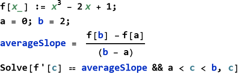
This confirms the existence of c and finds its exact value.

Rolle’s Theorem guarantees horizontal tangents when endpoints have equal values—useful for finding extreme values.

The Mean Value Theorem guarantees that the function cannot “skip” values in its average behavior—it must hit the average slope somewhere.

In physics they justify many approximations and existence results (e.g., that velocity must equal average velocity at some instant).

The Mean Value Theorem is a bridge between the local behavior of derivatives and the global behavior of functions. It is one of the deepest “existence” theorems in calculus and will appear again when we study Taylor series, integrals, and differential equations.

Exercise 20.21: Begin with Theorem 20.13 and copy it into your notebook. Reflect on its meaning for a few minutes. Note any thoughts that come to mind. How would you explain this to someone sitting in front of you. Write this down. Do this for each theorem, proof, and definition.

Exercise 20.22:
a) Consider the function on the interval [1, 3].
    1) Verify that f(1)=f(3).


    2) Use Rolle’s Theorem to guarantee the existence of a point c in (1, 3) where f'(c)=0.


    3) Find that point c explicitly.
b) Let on the interval [−2,2].
    1) Compute the average slope over [−2,2].
    2) Use the Mean Value Theorem to guarantee there is a point c in (−2,2) where f'(c) equals this average slope.
    3) Solve for c.
c) Apply the Mean Value Theorem to on the interval [1, 4].
    1) Find the value of c that satisfies the theorem.
    2) Verify that f'(c) really equals the average slope.
d) A car travels from rest at position s(0)=0 to s(4)=80 meters in 4 seconds, with position function .
    1) What is the average velocity over the 4-second interval?
    2) Use implicit differentiation with respect to time to find dV/dt.
    3) How fast is the radius changing at 5 seconds.
e) Consider the equation .
    1) Compute y'(x).
    2) Use the Mean Value Theorem to show there must be an instant when the instantaneous velocity equals this average.
    3) Find that exact instant.
f) Define f(x)=sin⁡ x on the interval [0,π].
    1) Compute the average slope over the interval.
    2) Use FindRoot or Solve in Wolfram Language to find the value(s) of c guaranteed by the Mean Value Theorem.
    3) Plot f(x) and the secant line from (0, f(0)) to (π,f(π)), and show the tangent line at c.
g) Explain in your own words the difference between Rolle’s Theorem and the Mean Value Theorem.
h) Why is the Mean Value Theorem sometimes called “the theorem that says a function must hit its average slope”?
i) Give a real-world situation (other than a car trip) where the Mean Value Theorem guarantees something must happen, even if we cannot easily measure it directly.

Proving Differentiability

We have spent considerable time learning how to compute derivatives using rules and shortcuts. Now we step back and ask a more fundamental question, “How do we prove that a function is actually differentiable at a particular point?” This brings us back to the rigorous definition we studied earlier. To prove that a function is differentiable at a point, we must show that the limit defining the derivative exists. In practice this often means simplifying the difference quotient until the limit becomes obvious. Proving differentiability is the bridge between the abstract definition and the practical rules we use every day. Sometimes the rules are enough; sometimes we must return to first principles.

A function f is differentiable at x=a if

(20.143)

exists (and is finite). To prove differentiability, we must evaluate this limit and show it is the same from both sides.

We do this by a method.

Write the difference quotient.

Simplify algebraically (expand, factor, rationalize, use trigonometric identities, etc.).

Take the limit as Δ x->0.

If the limit exists, the function is differentiable at a; the value of the limit is f'(a).

Worked ExamplesExample 1: A Polynomial (Easy Case)For example, we prove that the a specific polynomial is differentiable at x=1.

(20.144)

The difference quotient is,

(20.145)

Now take the limit

(20.146)

So f is differentiable at x=1 and f'(1)=5.

Now we check to see if f(x) = |x| is differentiable at x=0. The left-hand limit (Δ x->0-)

(20.147)

The right-hand limit (Δ x->0+)

(20.148)

The left- and right-hand limits are not equal, so the overall limit does not exist. Therefore f is not differentiable at x=0 (even though it is continuous there).

Let’s see if we can so a piecewise function

(20.149)

Let’s see if it is differentiable at x=1. First, check continuity: and the limit from right is 2(1)+1=3? So, actually this function is discontinuous at x=1, so it cannot be differentiable.

(Good counterexample practice.)Better Example: Adjust to a continuous piecewise function and show the derivative exists.

Use the rules whenever the function is built from differentiable pieces using sum, product, quotient, or chain rules. Use the definition when you have a piecewise function, absolute value, or need to prove differentiability from scratch (especially at “special points”).

Proving differentiability using the definition gives you confidence that the rules you have been using are built on solid ground. It also prepares you to handle more exotic functions that appear in advanced physics and analysis.

Exercise 20.23:
a) Prove is differentiable at x=2 and find f'(2).
b) Prove is differentiable at x=4 and find f'(4).
c) Consider the function,
    1) Prove this is differentiable at x=0.
    2) Find f'(0).
d) Explain the difference between continuity and differentiability. Give an example of a function that is continuous but not differentiable at a point.
f) Why is it important to be able to prove differentiability from first principles even when we have differentiation rules?

Summary

Write a summary of this chapter.

For Further Study

Silvanus Thompson, (1914), Calculus Made Easy. This is available for free at Project Gutenberg: https://www.gutenberg.org/files/33283/33283-pdf.pdf. This is a very elementary and nice introduction to calculus.

Jerrold E. Marsden, Alan Weinstein, (1985), Calculus I, II, and III. Springer-Verlag, New York. You can download it for free from CalTech: https://www.cds.caltech.edu/~marsden/volume/Calculus/

3Blue1Brown – “The paradox of the derivative” (Essence of Calculus, Chapter 2)
https://www.youtube.com/watch?v=9vKqVkMQHKk
The absolute best visual introduction to what a derivative really means. Grant Sanderson’s animations and deep insights make this unforgettable. Start here for intuition.

3Blue1Brown – “Derivative formulas through geometry” (Essence of Calculus, Chapter 3)
https://www.youtube.com/watch?v=FLAm7Hqm-58
Beautiful geometric explanations of the power rule, product rule, chain rule, and more. Pairs perfectly with your book’s approach.