Lesson 19 Interactivity in WL

“The joy of discovery is multiplied when you can immediately test your ideas and watch them unfold.” Grok

“Interactivity is the bridge between curiosity and understanding.” Grok

Introduction

Throughout this book we have built powerful tools—coordinate geometry, vectors, matrices, plotting, limits, and more. We can now describe motion, visualize functions, analyze limits, and model physical systems with precision. But something is still missing. Until now, most of our exploration has been somewhat static. We create a plot or run a calculation, look at the result, and then perhaps change a number and run it again.

In this lesson we cross an important threshold and learn how to make our mathematics and physics interactive. Instead of static pictures, we create living documents that respond immediately to our touch—where we can drag sliders, move points, change parameters in real time, and watch the physics unfold instantly. True understanding often comes not from observing, but from interacting. When you can change a parameter and immediately see the effect on a pendulum, a wave, or an electric circuit, intuition deepens dramatically. Interactivity turns passive learning into active discovery. It bridges the gap between theory and intuition by letting you play with mathematical and physical ideas in real time.In this lesson we will explore why interactive visualizations are so valuable in physics. You will learn the core interactive commands in Wolfram Language, especially Manipulate and Dynamic. We will build interactive models of simple harmonic motion, wave behavior, and the pendulum. You will discover how to create real-time data visualizations, use locators to drag points and watch equations update live, use the Tabular command to reproduce some aspects of spreadsheets, design custom graphical user interfaces, and even build an interactive circuit simulator. Finally, we will combine Manipulate and Dynamic, explore nested manipulations, and see how these tools open up entirely new ways of thinking about theoretical physics.

By the end of this lesson, your notebooks will no longer be static pages—they will become dynamic laboratories where ideas come alive at your fingertips. This is where computation stops being a calculator and starts becoming a true scientific companion.

Let us begin.

Why Interactive Visualizations are Important in Physics

We have spent many lessons learning to describe physical systems with equations, vectors, matrices, and plots. These tools are powerful, yet something is often still missing. A static graph or a single numerical result shows us what happens at one particular moment or under one set of conditions. It rarely shows us how the system responds when we change something.

True understanding in physics comes not just from observing a result, but from actively exploring how a system behaves when we vary its parameters in real time. Interactive visualizations transform passive observation into active discovery. They let us play with physics the way a musician plays with an instrument—changing one thing and immediately seeing (and feeling) the effect.

When you can drag a slider and instantly watch how the amplitude of a wave affects interference, or how changing the length of a pendulum alters its period, you begin to feel the relationships in your bones. You develop physical intuition far more rapidly than by studying static plots or solving equations alone.

Consider a simple pendulum. A static plot shows one trajectory. An interactive model lets you change the initial angle and watch how the motion evolves, adjust the length or gravity and see the period change instantly, explore large angles where the small-angle approximation breaks down.

Suddenly, abstract concepts like “restoring force proportional to displacement” become visceral. You don’t just know the mathematics—you feel the physics.

Interactive models often reveal surprises. You might notice a peak you didn’t expect, or discover that two seemingly different systems behave identically under certain conditions. These moments of discovery are where real learning happens.

In theoretical physics, we constantly move between idealized models and real-world behavior. Interactive visualizations serve as a bridge. They let you test the sensitivity of a model to parameters, explore limiting cases, and develop the judgment needed to know when a simplification is valid and when it is not.

As you gain experience with interactivity in Wolfram Language, you will find yourself thinking differently. Instead of asking “What is the answer?”, you will start asking “How does the system behave if I change this?” This shift in mindset is one of the hallmarks of a mature theoretical physicist.

In the sections that follow, we will learn the tools—Manipulate, Dynamic, locators, and more—that make this kind of deep, interactive exploration possible. Together, they will turn your notebooks into living laboratories for theoretical physics.

Interactive Commands in WL

We have seen why interactive visualizations are so powerful in physics. Now we begin learning how to create them. Wolfram Language provides a rich set of commands specifically designed for interactivity. These tools let you turn static calculations and plots into dynamic, responsive models that change in real time as you adjust parameters.

Instead of running a command once and getting one result, you can create an interface where changing a value instantly updates the output—whether it is a plot, a numerical result, or a physical simulation.

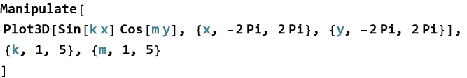
Manipulate is the workhorse of interactivity in Wolfram Language. It allows you to create sliders, buttons, and other controls that dynamically change parameters. In the book you will not see the value, you will have to duplicate it on your own.

Here, k becomes a controllable parameter with a slider. As you move the slider, the plot of sin⁡(kx) updates instantly.

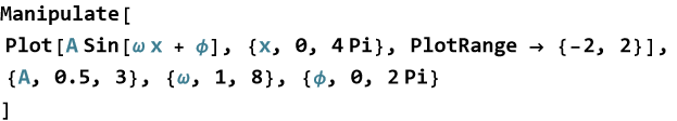
You can control several parameters at once.

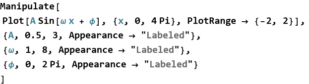
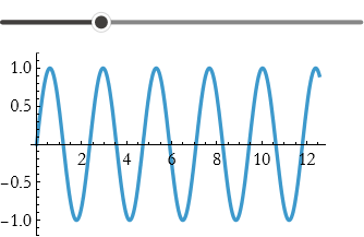
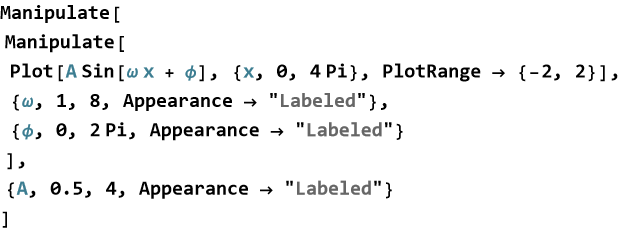
This creates a fully interactive model of a sine wave where you can adjust amplitude, frequency, and phase in real time.

Manipulate[]

We have seen how powerful interactivity can be for developing intuition in physics. Now we meet the single most important command that makes interactivity possible in Wolfram Language: Manipulate. Manipulate turns any expression—a plot, a calculation, a graphic, or even a table—into a living document that responds instantly as you adjust parameters with sliders, checkboxes, menus, or other controls. Manipulate lets you explore “what if?” questions in real time. Change a value, and the entire output updates immediately. This is where theoretical physics becomes experimental in the best sense. The simplest Manipulate looks like this.

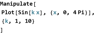
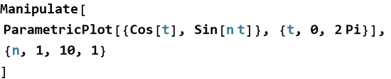
Here {k, 1, 10} creates a slider for the parameter k. Move the slider and watch the frequency of the sine wave change instantly.

Manipulate can control almost anything you can compute in Wolfram Language.

3D Surfaces.

Parametric Curves and Animations.

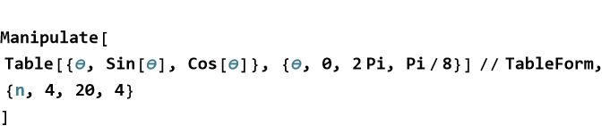
Numerical Results and Tables.

Manipulate supports many control types:

Slider (default): {var, min, max}
Checkbox: {var, {False, True}}
PopupMenu / Dropdown: {var, {value1, value2, ...}}
RadioButton: {var, {choice1, choice2, ...}}
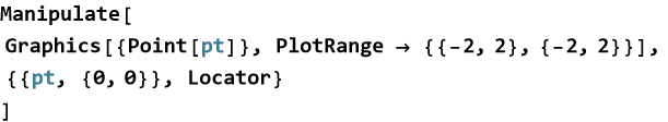
Locator (drag points on a graph).

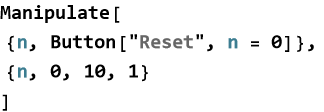
Button (for actions).

CheckBox:

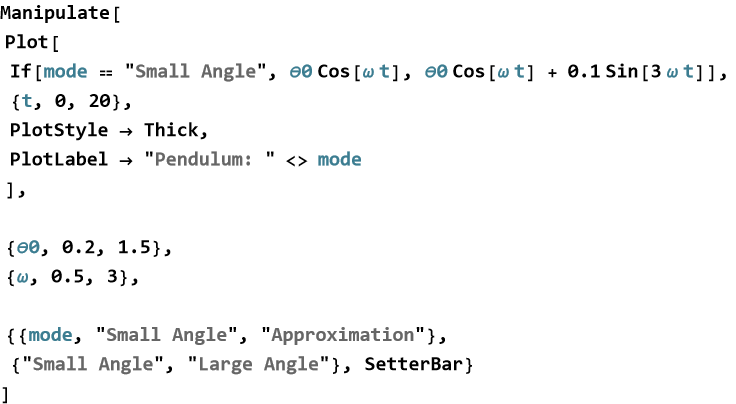
A SetterBar lists options.

Slider2D

Exercise 19.1:
a) Create a Manipulate that plots y=A sin⁡(x) where the amplitude A can be varied from 0.5 to 5 using a slider. Add a meaningful label and appropriate PlotRange.
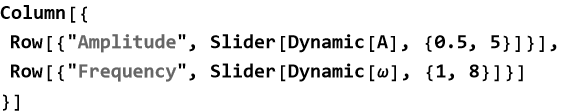
b) Build an interactive sine wave model with three controls:
    Amplitude A (0.5 to 4)
    Angular frequency ω (0.5 to 8)
    Phase shift φ (0 to 2π)
    Use labeled sliders and a good PlotLabel.
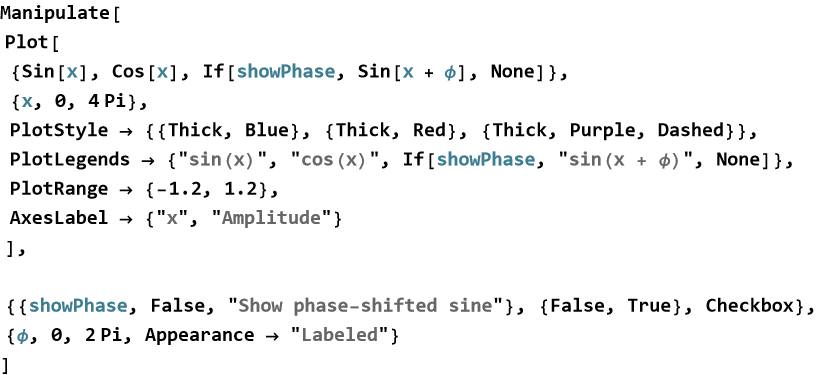
c) Create a Manipulate that shows both sin⁡(x) and cos⁡(x). Add a checkbox labeled “Show Sum” that toggles the display of sin⁡(x)+cos⁡(x).
d) Make an interactive plot that lets the user choose between different functions using a SetterBar: sin (x), cos (x), sin (2 x).

Simple Harmonic Motion

We have explored oscillations and built interactive tools in Wolfram Language. Now we focus on one of the most important and elegant types of motion in all of physics, simple harmonic motion (SHM). We are not new to this kind of motion. This occurs when the restoring force is directly proportional to the displacement from some equilibrium position that always seems ro be opposite in direction, the resulting motion is simple harmonic. This is the “purest” form of oscillation—smooth, predictable, and mathematically beautiful. It serves as a foundation for understanding more complicated real-world vibrations.

For a mass on a perfect spring, the position as a function of time is

(19.1)

where A is the amplitude (the maximum vertical displacement), ω=k/m is the angular frequency where k represents the strength of the spring and m the mass of the oscillator, and φ is the phase constant. The velocity and acceleration follow naturally ( as we will see in in the next lesson,

(19.2)

(19.3)

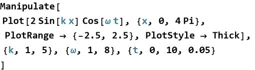
Here is a powerful interactive model you can experiment with.

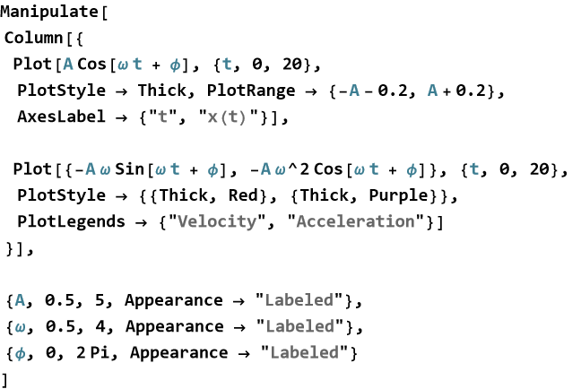
Move the sliders and watch how amplitude, frequency, and phase affect the motion. Notice that velocity leads position by 90°, and acceleration is always opposite to position.

A particularly insightful view comes from plotting position versus velocity parametrically.

This produces a beautiful ellipse in phase space—a hallmark of simple harmonic motion and a visual proof of energy conservation.

Simple harmonic motion is not just a mathematical curiosity. It appears everywhere in nature and technology: tuning forks, clocks, electrical circuits, molecular vibrations, and even the small vibrations of bridges and buildings. Mastering it gives you deep insight into oscillatory systems across all of physics.

Exercise 19.2:
a) The position of a harmonic oscillator is given by x(t)=4cos⁡(3t) meters.
    1) Plot x(t) for t from 0 to 10 seconds.
    2) On the same graph, plot the velocity v(t)=−12sin⁡(3t) m using a different color and add a legend.
    3)  Describe the phase relationship between position and velocity.
    4) Use ParametricPlot with AspectRatio -> Automatic to create a parametric plot of position versus velocity.
    5) Add appropriate labels and a title.
    6) Explain what the shape of this plot tells you about the total mechanical energy of the system.
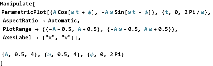
b) Create a Manipulate for a general harmonic oscillator x(t)=A cos⁡(ω t+φ). Include sliders for amplitude A (0.5 to 5), angular frequency ω (0.5 to 6), and phase φ (0 to 2π).
c) What is the physical significance of the elliptical trajectory in the phase space plot?

Wave Behavior

We have explored simple harmonic motion and built interactive models that respond in real time. Now we take the next natural step, waves. A wave is a disturbance that travels through space or a medium, transferring energy from one place to another without permanently moving the medium itself. Waves are propagating oscillations. They combine the back-and-forth motion we saw in simple harmonic oscillators with the idea of travel through space. A wave is what happens when simple harmonic motion moves from one location to the next.

A simple traveling wave moving to the right can be described by

(19.4)

note that this is a function of two variables, position x and time t, where A is the amplitude, k=2π λ is what we call the wave number and represent show many waves can fit in a cycle, λ is the wavelength, ω=2π f is the angular frequency (f is the frequency), and φ  is the phase constant.

You can visualize a traveling wave interactively.

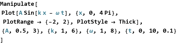
As you adjust the parameters, watch how the wave propagates.

When two or more waves overlap in the same region, their displacements add together. This is called superposition. The result can be constructive interference (waves reinforce each other) or destructive interference (waves cancel each other).

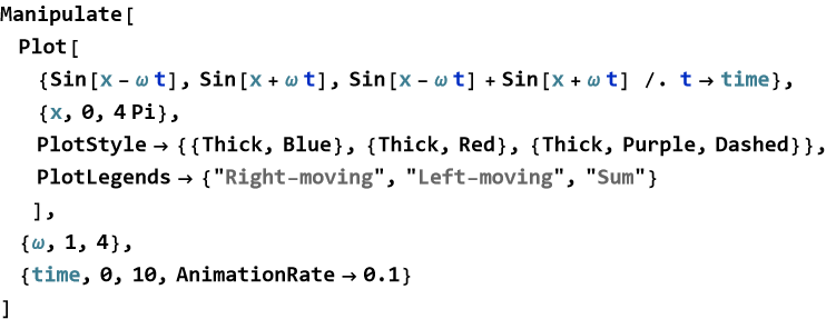
This is weird, it only shows the sum. Let’s try wrapping each Sin in an Evaluate.

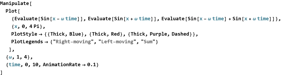
This worked.

This interactive model beautifully demonstrates how two traveling waves can combine to form a standing wave when they have the same frequency.

Recall that a standing wave is a special pattern that appears to stand still while the medium oscillates up and down. It is formed by the interference of two identical waves traveling in opposite directions.

Notice the fixed nodes (points that never move) and antinodes (points of maximum oscillation).

Wave behavior is fundamental to understanding sound, light, water waves, seismic waves, and even quantum mechanics. By building and interacting with these models, you develop an intuitive feel for how waves propagate, interfere, and form standing patterns.

Exercise 19.3:
a) A traveling wave is described by y(x,t)=3sin⁡(2x−4t).
    1) Plot the wave at t=0 and at t=π/4 on the same graph using different colors.
    2) Use Manipulate to create an interactive version where you can vary time t.
b) A standing wave is given by y(x,t)=4sin⁡(2x)cos⁡(3t).
    1) Plot this function for a fixed time.
    2) Use Manipulate to animate the standing wave.
    3) Mark the locations of nodes and antinodes on your plot and explain their physical meaning.
c) Build a Manipulate with two waves of the same amplitude but controllable phase difference.
    1) Include a slider for the phase difference Δ φ.
    2) Plot both individual waves and their superposition.
    3) Find the values of Δ φ that produce perfect constructive and perfect destructive interference.
d) A wave is described by y(x,t)=2sin⁡(k x−ω t).
    1) Create an interactive Manipulate with sliders for k and ω.
    2) Calculate the wave speed v=ω/k and display it as a labeled value in the Manipulate.
    3) Experiment with different values and describe how changing k and ω affects wavelength, frequency, and speed.
e) Explain in your own words the difference between a traveling wave and a standing wave.
f) How does superposition lead to the formation of standing waves?

The Pendulum

One of the most iconic examples of oscillatory motion is the simple pendulum—a mass suspended from a fixed point that swings back and forth under gravity. It appears in clocks, scientific instruments, and even our intuitive understanding of periodic motion. While we briefly met the pendulum earlier, we now explore it more deeply using the interactive tools we have developed. For small angles, the pendulum behaves like a simple harmonic oscillator. For larger angles, the motion becomes richer and more complicated. The pendulum beautifully illustrates how a constant force (gravity) can produce periodic motion, and how approximations affect our description of reality.

For small angular displacements θ, the equation of motion approximates simple harmonic motion

(19.5)

where l is the length and g is the acceleration due to gravity. Here is an interactive model.

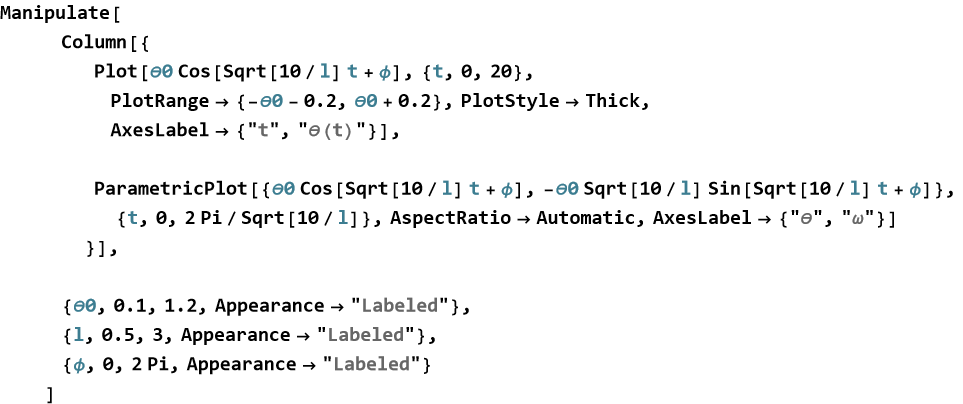
For larger angles, the motion is no longer purely sinusoidal. The period increases slightly, and the waveform becomes more flattened at the peaks. You can explore this by comparing the small-angle approximation with the numerical solution of the exact pendulum equation, we will explore this in later lessons and volumes.

The pendulum is far more than a toy. It is a gateway to understanding periodic motion, small-angle approximations, and the transition from linear to nonlinear dynamics—concepts that appear throughout classical and quantum physics.

By building and playing with interactive pendulum models, you gain both mathematical insight and physical intuition that will serve you well in the chapters ahead.

Exercise 19.4:
a) A simple pendulum of length l=1 m has small angular displacement given by θ(t)=0.5cos⁡(g/l t), where g=9.8 . Plot θ(t) for t from 0 to 20 seconds.
b) Create a Manipulate for a simple pendulum using the small-angle approximation . Include sliders for initial angle (0.1 to 1.0 rad) and length l (0.5 to 3 m).
c) Explain in your own words why the simple pendulum is such an important example in classical mechanics.

Dynamic[]

We have seen how Manipulate creates powerful interactive demonstrations by letting you control parameters with sliders and other controls. But sometimes you want something even more responsive—a value or graphic that updates continuously and instantly as variables change, without needing a separate “evaluate” step. This is where the command Dynamic shines. Dynamic turns any expression into a live, continuously updating object. As soon as a variable it depends on changes, the expression re-evaluates automatically. While Manipulate builds interactive interfaces, Dynamic creates truly live content that responds in real time.

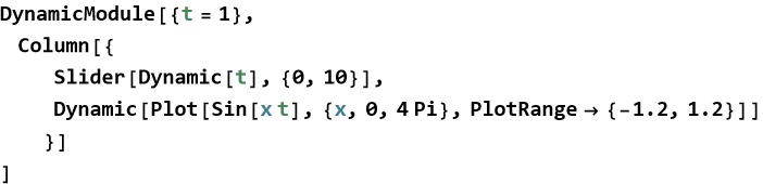
The simplest use of Dynamic is to display a value that updates live.

Now move a slider connected to x.

As you drag the slider, the number updates immediately.

Dynamic becomes especially powerful when combined with graphics.

Or with a live plot.

You can combine both for maximum flexibility.

Use Dynamic when you want:

Real-time updating text or numbers

Graphics that respond instantly

Live calculations that change as parameters are adjusted

More responsive behavior than Manipulate alone provides

Dynamic is one of the most elegant and powerful features in Wolfram Language. It turns your notebooks into responsive scientific instruments.

Mastering Dynamic alongside Manipulate gives you the ability to build rich, professional-quality interactive models for exploring physics.

Exercise 19.5:
a) Define a variable x and create a live display using Dynamic.
    1) Show Dynamic[x] next to a slider that controls x from 0 to 10.
    2) Add a second Dynamic that shows .
    3) Explain why the displayed values update instantly as you move the slider.
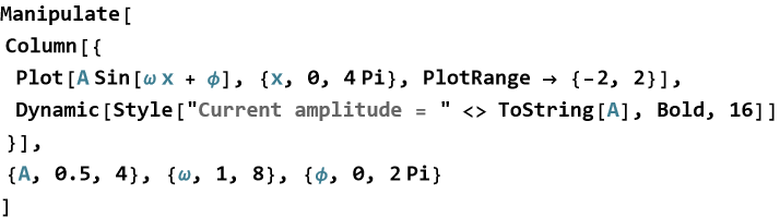
b) Create a Manipulate that controls a parameter A.
    1) Use Dynamic to display a live label such as “Current amplitude = “ followed by the value of A.
    2) Plot A sin⁡(x) on the same interface.
    3) What advantage does using Dynamic for text provide over static labels?
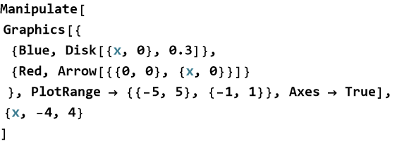
c) Create an interactive model of a moving particle.
    Manipulate[
         Graphics[{
           {Blue, Disk[{t, Sin[t]}, 0.2]},
           {Red, Arrow[{{0, 0}, {t, Sin[t]}}]}
          }, PlotRange -> {{0, 10}, {-1.5, 1.5}}, Axes -> True],
         {t, 0, 10, 0.05}
        ]
    1) Replace the static t with Dynamic[t] inside the Graphics.
    2) Observe the difference in behavior.
    3) When is using Dynamic inside graphics particularly useful?
d) Build a Manipulate for a harmonic oscillator x(t)=Acos⁡(ω t).
    1) Use Dynamic to display the current period T=2π/ω in real time.
    2) Also display the maximum velocity .
    3) Explain how Dynamic makes numerical feedback more effective than static text.
e) Create an interface with:
    A slider for frequency ω
    A checkbox to toggle between sine and cosine
    A live Dynamic display showing the current function being plotted
    Plot the selected wave with Dynamic updating smoothly.
f) Explain in your own words the difference between Manipulate and Dynamic.
g) Why does combining Manipulate and Dynamic create more powerful interactive tools than using either alone?

Real-Time Data Visualization

We have learned how to create static plots and interactive models that respond to sliders. The next level of visualization is to watch data evolve in real time—as if you were monitoring a live experiment. Real-time data visualization lets you see quantities changing continuously, much like watching a live oscilloscope or a sensor readout in a laboratory. So, instead of plotting a fixed dataset once, you can create plots and displays that update automatically as new data arrives or as simulated quantities change over time. Real-time visualization turns your notebook into a dynamic instrument—a digital laboratory where you can observe physical processes as they unfold.

The simplest way to create real-time behavior is to combine Dynamic with a time-dependent expression.

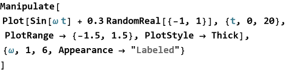
This creates a noisy sine wave that updates continuously as time progresses.

You can simulate monitoring a signal, such as voltage in an electrical circuit.

In experimental and theoretical physics, many phenomena are inherently time-dependent. Being able to watch a system evolve in real time helps you:

Spot unexpected behavior immediately,

Develop intuition about rates of change,

Compare theory with simulated or real measurements dynamically,

Build more engaging demonstrations and teaching tools.

Real-time data visualization is one of the most exciting capabilities of Wolfram Language. It transforms your computer from a calculator into a live scientific instrument.

Exercise 19.6:
a) Create a Manipulate that shows a noisy sine wave updating in real time.
    1) Plot y=sin⁡(3t)+0.3 random noise.
    2) Use Dynamic or appropriate Manipulate controls to make the wave evolve as time progresses.
    3) Add a live display of the current time using Dynamic.
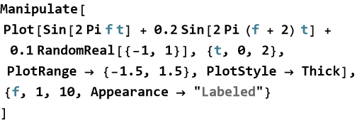
b) Build a simple interactive “oscilloscope” that displays a signal of the form V(t)=A sin⁡(2π f t+φ)+noise.
    1) Use Manipulate with sliders for amplitude A, frequency f, and phase φ.
    2) Make the plot update in real time as if scanning across the signal.
    3) Add a Dynamic display showing the current frequency in Hz.
c) Explain in your own words why real-time data visualization is more powerful than static plots for understanding physical systems.
d) Describe one situation in physics (mechanics, waves, circuits, thermodynamics, etc.) where real-time visualization would be especially helpful.
f) What are the advantages and limitations of using Dynamic and Manipulate for real-time simulations?

Tabular[]

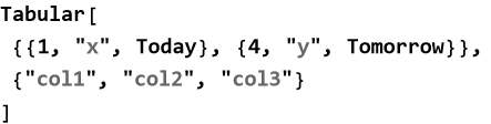
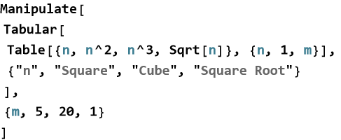
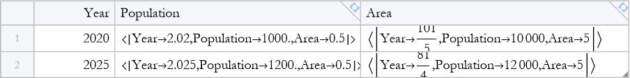
In addition to Grid and Dataset, Wolfram Language provides a modern and convenient way to create well-formatted tables with Tabular. This command is especially useful when you want clean, labeled tables with proper column headers and good default styling that have some features of spreadsheets. Tabular takes structured data (matrices, associations, or lists of columns) and automatically produces a nicely formatted table with column names when provided. Tabular gives you beautiful, publication-ready tables with minimal effort.

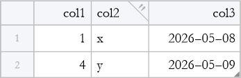
Creating a Tabular object from a matrix.

With column keys.

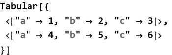
From a list of associations (very powerful).

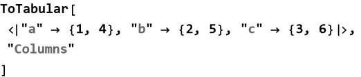
From column data.

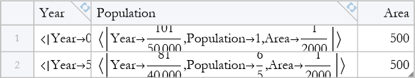
You can also create a Tabular object directly from a Dataset.

Interactive Table.

Tabular is a welcome addition to Wolfram Language’s data presentation tools. Use it whenever you want to display structured numerical or categorical data in a clean, readable format — especially in reports, demonstrations, or interactive models.

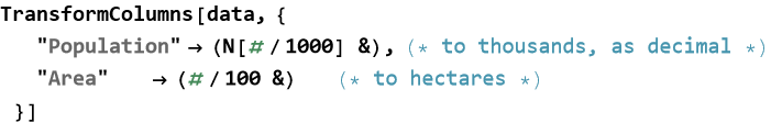
Once you have created a Tabular object or a Dataset, you often need to modify the data in specific columns—for example, converting units, applying a mathematical function, or formatting numbers. The command TransformColumns is designed exactly for this purpose.TransformColumns lets you apply a transformation (a function) to one or more columns of a table while leaving the rest of the data unchanged. Instead of rewriting an entire table, you can selectively transform individual columns in a clean and readable way.

Applying a function to a column.

Multiple transformations.

You can also add new columns by assigning to a new key.

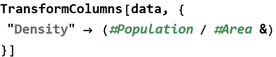
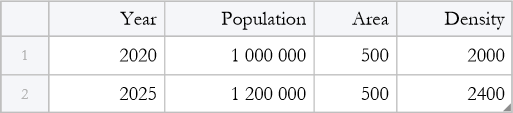
This creates a new column called "Density".

TransformColumns is one of the most practical tools for working with structured data in Wolfram Language. Mastering it will make your data analysis and presentation much more efficient.

How Dragging Points can Change an Equation

We have seen how sliders and checkboxes let us explore mathematical ideas interactively. Now we take interactivity to an even more intuitive level, where dragging points directly on a graph and watching an equation update in real time. So instead of typing numbers, you can literally point at the graph, drag points with your mouse, and see the best-fit equation or curve adjust instantly. This creates a direct, tactile connection between data and mathematics. Dragging points turns curve fitting from an abstract calculation into a hands-on experience—you move the data, and the equation follows.

The key option for a Manipulate for this is Locator. Here is a simple example where you can drag two points and see the line connecting them.

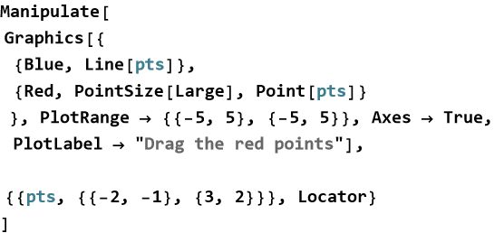
A much more powerful application is to fit a mathematical model to the points you drag.

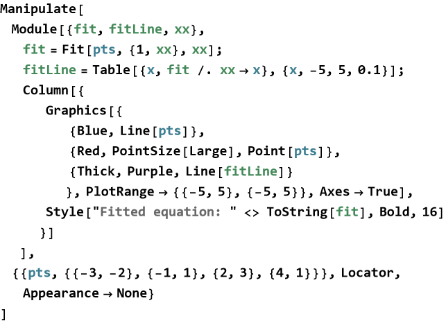
As you drag the red points, the purple best-fit line and its equation update immediately.

You can simulate experimental data and fit a quadratic trajectory.

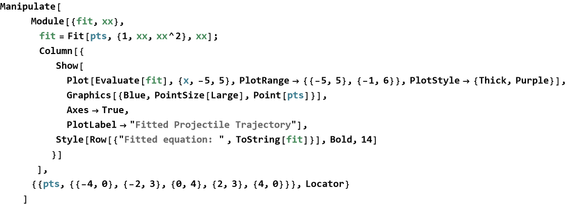
This lets you explore how well a quadratic model fits “experimental” data by dragging the points.

By combining locators with fitting, you turn your notebook into an interactive laboratory where data and theory meet in real time.

GUI Design in WL without Manipulate

We have seen how Manipulate provides quick and powerful interactivity. However, sometimes you need more control over the layout, behavior, or appearance of your interface. In these cases, you can build custom graphical user interfaces (GUIs) directly using lower-level Wolfram Language tools. This gives you greater flexibility and deeper understanding of how interactivity works. You can create rich, custom interfaces by combining DynamicModule, Dynamic, controls (Slider, Button, Locator, etc.), and layout functions (Column, Row, Grid, Panel). Building a GUI without Manipulate is like moving from using a ready-made toolbox to designing and building the toolbox yourself.

DynamicModule creates a localized, self-contained dynamic environment. It is the recommended starting point for custom interfaces.

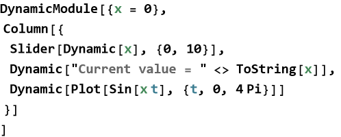
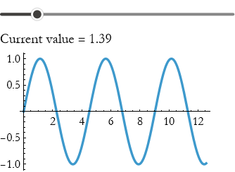
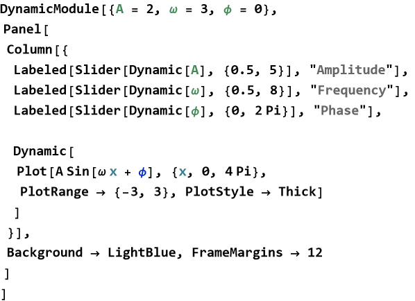
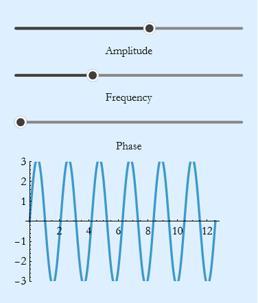
Here is a more complete example—a custom control panel for a harmonic oscillator.

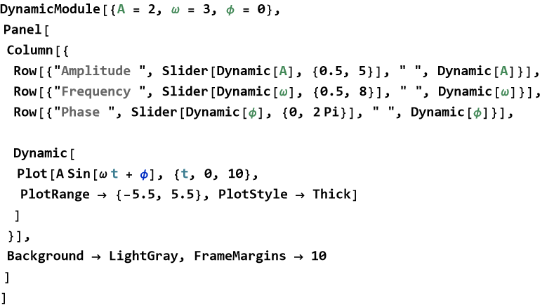
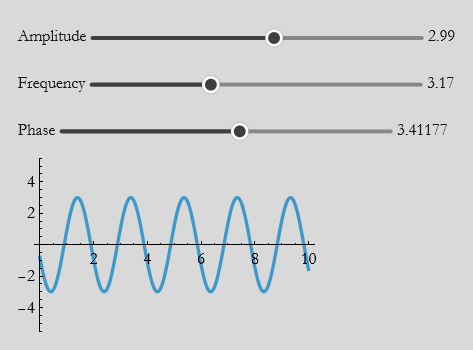
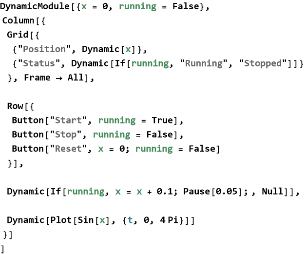
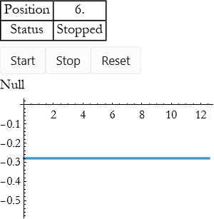
You can create more sophisticated interfaces using Grid, Button, and other controls.

Why Build GUIs without Manipulate?

Greater control over layout and appearance

Ability to create complex, multi - panel interfaces

Better performance for advanced applications

Deeper understanding of how Wolfram Language handles dynamics

Suggested Activity
Design your own custom interface for one of the physical systems you have studied (a pendulum, wave interference, RC circuit, or projectile motion).

Use DynamicModule, Dynamic, and layout functions to create sliders, buttons, and live plots. Focus on making the interface clear and educational for someone learning the topic.

Building custom GUIs without Manipulate gives you the freedom to create exactly the interactive experience you want. It is a powerful skill that will serve you well as you develop more sophisticated demonstrations and tools in theoretical physics.

WL GUI Commands

We have seen how Manipulate and Dynamic allow us to create powerful interactive models. As your interfaces become more sophisticated, you will want finer control over layout, appearance, and user interaction. Wolfram Language provides a rich collection of GUI (Graphical User Interface) commands that let you build custom, professional-looking interfaces from the ground up. You can combine basic building blocks—panels, buttons, sliders, layouts, and dynamic elements—to create exactly the interactive experience you need for exploring physics. Learning individual GUI commands gives you the freedom to design interfaces that feel natural and educational, rather than being limited to the default style of Manipulate.Core

Panel —Creates a framed, visually distinct region.

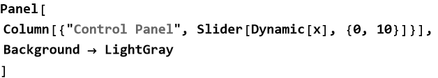
Column and Row—Organize elements vertically or horizontally.

Grid—Creates structured tables or control layouts with precise alignment.

Button—Performs an action when clicked.

You can wrap almost any GUI element with Dynamic to make it live.

For example,

WhMastering individual GUI commands gives you:

Complete creative freedom over layout and design

Better performance for complex interfaces

The ability to create polished demonstrations and teaching tools

A deeper understanding of how interactivity works in Wolfram Language

Suggested Activity
Design a small custom interface for one of the physical systems you have studied (a pendulum, wave interference, or RC circuit). Use DynamicModule, Panel, Column, sliders, and Dynamic to create a clean, educational control panel. Focus on making it intuitive for someone learning the topic for the first time.

As you become comfortable with these GUI commands, you will be able to create rich, professional-quality interactive tools that greatly enhance both your own learning and your ability to communicate ideas in theoretical physics.

Nested Manipulations

We have seen how Manipulate lets us create rich interactive models by controlling parameters with sliders and other tools. As your explorations become more sophisticated, you will often want to organize complicated interfaces with multiple levels of control. This is where nested manipulations become extremely powerful. You can place one Manipulate (or Dynamic expression) inside another, or combine multiple interactive elements in a structured way. This allows you to create hierarchical, well-organized interfaces that are both powerful and easy to use. Nested manipulations let you build interfaces with clear logical structure—separating global controls from local ones, or organizing related parameters into groups.

Here is a simple example where an outer Manipulate controls the overall behavior, while an inner one fine-tunes a detail.

The outer slider controls amplitude, while the inner controls allow detailed adjustment of frequency and phase.

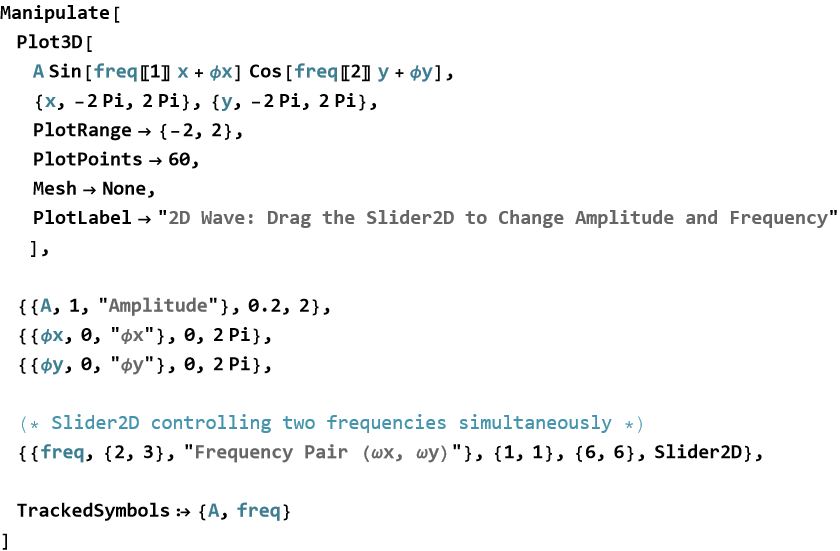
A more sophisticated nested example — controlling a wave system.

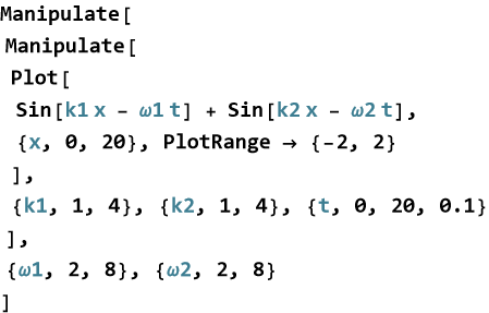
The outer controls set the overall frequency range, while the inner Manipulate lets you explore time evolution and wave numbers in detail.

When to Use Nested Manipulations

When you have both global and local parameters

When you want to organize a complex interface into logical groups

When building educational tools with different levels of detail

When combining different types of visualizations (plot + table + numeric display)

Suggested Activity
Design a nested Manipulate for one of the physical systems you have studied (for example, a pendulum with controls for length, gravity, and initial angle at the outer level, and damping or driving force at the inner level). Pay attention to how the organization of controls affects usability. A well-designed nested interface feels natural and helps the user focus on the physics rather than the controls.

Nested manipulations are one of the more advanced yet highly rewarding techniques in Wolfram Language. They allow you to create professional-quality, well-structured interactive demonstrations that greatly enhance both your own exploration and your ability to communicate ideas in theoretical physics.

Summary

Write a summary of this lesson.

For Further Study

Sal Mangano, (2010), Mathematica Cookbook, O’Reilly Media Inc. Has an extensive chapter on interactivity.

Manipulate: The Ultimate Interactive Tool (Highly Recommended)By: Wolfram Research (Official)
Excellent introduction to Manipulate with many practical examples.

Dynamic and Manipulate in Wolfram LanguageBy: The Math Sorcerer
Clear, step-by-step tutorial covering both Manipulate and Dynamic.

Advanced Manipulate TechniquesBy: Wolfram Research
Covers nested Manipulate, performance tips, custom controls, and DynamicModule.

Building Custom GUIs in Wolfram Language (without Manipulate)By: Various Wolfram developers / community experts
Focuses on DynamicModule, Panel, Locator, buttons, and custom layouts.