Lesson 20 Calculus 1 Limits and Continuity

“The limit is the bridge between the finite and the infinite.”  Inspired by the spirit of calculus.

“Calculus is the mathematics of change, and limits are its foundation.” Common teaching wisdom.

Introduction

We have spent many lessons building a strong foundation in algebra, geometry, vectors, matrices, and visualization. Now we take a major step forward into the mathematics of change. Calculus is the language that describes how quantities vary—how position becomes velocity, how velocity becomes acceleration, and how functions behave as we zoom in closer and closer to a point.

At the heart of calculus lie two closely related ideas, limits and continuity. They tell us what happens as we approach a value without necessarily reaching it, and whether a function behaves smoothly or has sudden jumps.The central idea of this lesson is that even though we cannot always reach a certain point exactly, we can get as close as we like and still make reliable statements about what happens there. Limits give us the precision to talk about “approaching,” and continuity tells us when a function has no breaks or jumps.

Limits and continuity are the tools that let us handle the infinite and the infinitesimal in a rigorous yet intuitive way.

In this lesson we will explore the formal epsilon-delta definition of limits, develop a visual understanding of what limits mean, study the properties of limits, and learn how to prove them. We will examine one-sided limits, limits at infinity, and how continuity is defined using limits. You will see powerful theorems such as the Intermediate Value Theorem and learn how to use Wolfram Language to visualize and confirm continuity.

By the end of this lesson you will have the foundational tools of calculus. You will be able to talk confidently about approaching values, determine whether functions are continuous, and prepare for the study of derivatives and integrals that follow. This is where the real power of theoretical physics begins to unfold.

Let us begin our journey into the mathematics of change.

Epsilon-Delta Definition of Limits

Up to now we have worked with functions where we could simply plug in a value of x and get a result. But sometimes we want to know what happens as x gets closer and closer to a particular number a, even if we never actually reach a. We say that the function approaches a certain value L, the limit of the function,  as x approaches a. This idea of “approaching” is at the heart of calculus.

Even if a function is not defined at a point, or behaves strangely exactly at that point, we can still make precise statements about what value it gets arbitrarily close to.

Limits let us talk rigorously about what a function does as we get closer and closer to a value without necessarily reaching it.

We say

(18.1)

if, as x gets closer and closer to a (from both sides), the value of f(x) gets closer and closer to L.

To make this idea completely rigorous, mathematicians use something called the epsilon-delta notation to define the limit precisely.

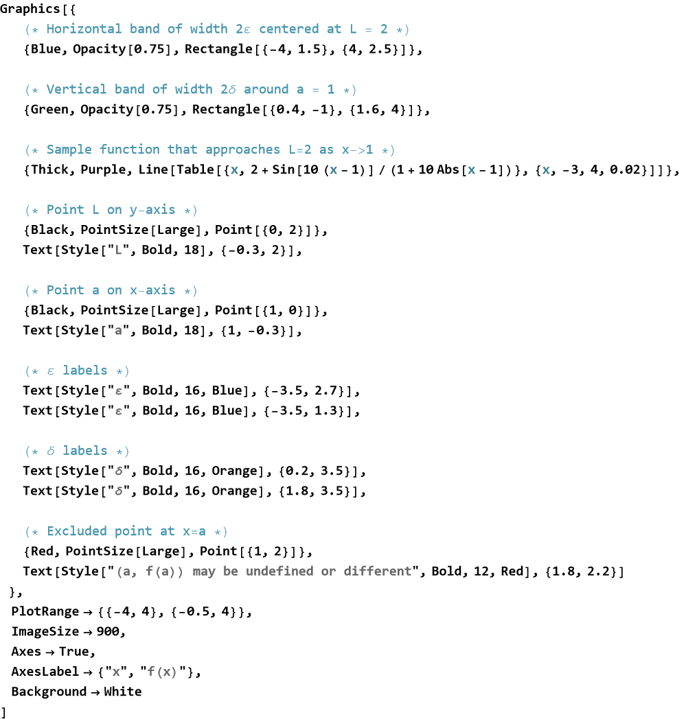
Definition 18.1 Epsilon-Delta Definition of a Limit: We say that the limit of f(x) as x approaches a is L as described in (18.1) above, if for every positive number ε>0 (this represents our tolerance for how close the output must be to L) there exists a positive number δ>0  (this represents how close x must be to a) such that

(18.2)

In plain language we say that no matter how small an error tolerance ε you choose around the target value L, you can always find a small enough region around a (excluding a itself if necessary) where the function stays inside that tolerance.

This definition may feel formal at first, but it is the foundation that makes all of calculus rigorous. It allows us to prove statements about limits with complete certainty.

Definition 18.2 Epsilon-Delta Notation (Weierstrass–Jordan Criterion): The epsilon-delta notation, also known as the Weierstrass–Jordan criterion, is the precise mathematical language used to define limits. It gives us a rigorous way to say that a function gets arbitrarily close to a value L as the input x gets arbitrarily close to a, without ever having to reach a. Formally, we write (18.1) if and only if for every positive number ε>0 (the tolerance in the output), there exists a positive number δ>0  (the tolerance in the input) such that (18.2) holds true.

No matter how small an error you are willing to accept around the target value L (that is your ε), you can always find a small enough neighborhood around a (controlled by δ) where the function stays inside that error band — except possibly right at the point x=a itself.

This notation was developed by mathematicians such as Karl Weierstrass and Camille Jordan to make the intuitive idea of “approaching” completely rigorous. It is the foundation of modern calculus.

Definition 18.3 Neighborhood of a Point: Let a be a real number and let δ>0 be a positive real number. There is an open interval around a that we call the neighborhood of a where the radius is  δ . It is written as (a−δ,a+δ)or{x∈R∣0<∣x−a∣<δ}.

A neighborhood is a small open interval around the point a. It tells us how close we are willing to get to a without actually touching it.

This concept is essential in the epsilon-delta definition of limits. When we say “there exists a δ>0 such that (18.2) holds...”, we are choosing a neighborhood around a small enough to guarantee that the function values stay within the desired tolerance ε.

No matter how small a tolerance ε we choose for the output, we can always find a small enough neighborhood around the input point a where the function behaves as desired.

The epsilon-delta definition gives us a precise language for talking about approaching values. It is the bedrock upon which the entire structure of calculus — derivatives, integrals, continuity, and more — is built.

Take your time with this concept. It may feel abstract now, but it will become one of your most reliable tools as we move forward.

Exercise 18.1: Begin with Definition 18.1 and copy it into your notebook. Reflect on its meaning for a few minutes. Note any thoughts that come to mind. How would you explain this to someone sitting in front of you. Write this down. Then do this for each definition.

Properties of Limits

Now we know what a limit is and how the epsilon-delta definition makes it precise. Once we accept that limits exist, a wonderful thing happens, we find that they behave in very predictable and useful ways. These predictable behaviors are called the properties of limits.The central idea is that limits respect the ordinary operations of arithmetic. If two functions have limits, then their sum, difference, product, and quotient (when defined) also have limits—and we can find those limits easily.

Limits turn complicated problems into simpler ones by letting us work with the limiting values directly.

Assume that the following limits exist

(18.3)

(18.4)

Then the following properties hold.

Theorem 18.1 Sum Rule:

(18.5)

Theorem 18.2 Difference Rule:

(18.6)

Theorem 18.3 Constant Multiple Rule:

(18.7)

Theorem 18.4 Product Rule:

(18.8)

Theorem 18.5 Quotient Rule (provided M≠0):

(18.9)

Theorem 18.6 Power Rule: For any positive integer n

(18.10)

Theorem 18.7 Root Rule: For any positive integer n

(18.11)

(when the root is defined).

These properties allow us to break complicated limits into simpler pieces we already know how to evaluate.

The properties of limits are what make calculus practical. Instead of struggling with the full epsilon-delta argument every time, we can use these rules to compute limits quickly and confidently. They are the everyday tools you will reach for again and again as you study calculus and applications in physics.

Epsilon-Delta Proofs

We have stated the seven important properties of limits. Now we prove them using the epsilon-delta definition. This is the moment when the precise language we learned earlier shows its true power.

Once we accept the epsilon-delta definition as the rigorous meaning of a limit, every property we use must follow logically from that definition. Proving the properties gives us complete confidence that the rules we rely on every day are actually true. Each proof shows that if the individual limits exist, then the combined expression also satisfies the epsilon-delta condition.

Proving a limit using the epsilon-delta definition can seem intimidating at first, but it follows a reliable pattern. Once you learn this pattern, most proofs become systematic.

Here are the main steps in such a proof:

State clearly what you intend to prove. For example, “We will show that ”

Let ε>0 be given.

Express the conclusion you need to get to. For example, “You need |f(x) − L| < ε.” This allows you to work backwards.

Start by writing the inequality and simplifying it, if necessary. For example we have |f(x) − L|, and we can simplify it in terms of |x − a|.

Manipulate the inequality.

Factor or bound |f(x) − L| so that it contains a factor of |x − a|.

Often you will get something like |f(x) − L| ≤ K |x − a| (or similar), where K is some constant that may depend on a but not on ε.

If the expression is more complicated (square roots, rationals, etc.), you may need to restrict δ in advance (e.g., assume δ ≤ 1) to get useful bounds.

If the function is a polynomial or rational, factor it.

For roots or fractions, multiply by conjugates or use inequalities like .

Choose δ. Solve for the δ that makes your bound less than ε. Typical choices are δ = ε / K (if you have |f(x) − L| ≤ K |x − a|) or we pick the smaller of a set of numbers, called  min, δ = min{1, ε / K} (when you need to restrict the neighborhood first). When the expression blows up near a, you often restrict δ ≤ some number (e.g., δ ≤ 1) to keep x away from the blow up point, what we call singularities.

Assume 0 < |x − a| < δ. Show the algebraic steps that lead to |f(x) − L| < ε. For example, you can end with, “Therefore, by the ε - δ definition, the limit is L.”

We will prove the seven rules one by one. The proofs for the first few are straightforward; the later ones are a bit more subtle but follow the same logical pattern.

Theorem 18.1 Sum Rule:

Step-by-Step ε-δ Proof:

Let ε > 0 be given (arbitrary). We need to find δ > 0 such that if 0 < |x − a| < δ, then |f(x) + g(x) − (L + M)| < ε.

Step 1: Start with the expression we must control,

(18.12)

The triangle inequality is the key tool here.

Step 2: We want the sum of the two tolerances to be less than ε. A simple way is to make each error less than ε/2. Let and . (Note: and are both positive because ε > 0.)

Step 3: Because , there exists such that if , then . Similarly, because , there exists such that if , then .

Step 4: We define delta = . (This is positive because both and are positive.)

Step 5: Assume 0 < |x − a| < δ. Then and . Therefore, |f(x) − L| < ε/2 and |g(x) − M| < ε/2. Adding these gives

(18.13)

Thus, by the ε-δ definition, . QED

Theorem 18.2 Difference Rule:

Step-by-Step ε-δ Proof:

Let ε>0 be given (our arbitrary positive tolerance). Since , there exists such that if , then .Since , there exists such that if , then |g(x)−M∣<ε2.

Now choose

(18.14)

Assume 0<∣x−a∣<δ. Then both conditions above are satisfied, so

(18.15)

Using the triangle inequality,∣

(18.16)

Therefore, by the definition of the limit, This completes the proof. QED

Theorem 18.3 Constant Multiple Rule:

Step-by-Step ε-δ Proof:

Let ε>0 be given (our arbitrary positive tolerance for the output). We need to find a δ>0 such that if 0<∣x−a∣<δ, then

(18.17)

First, simplify the expression we want to control

(18.18)

We want this to be less than ε

(18.19)

(If c=0, the result is trivial since both sides are zero. Assume c≠0.)

Because, there exists a δ>0 such that, if 0<∣x−a∣<δ, then

(18.20)

Choose exactly this same δ.Then, whenever 0<∣x−a∣<δ, we have

(18.21)

This is precisely what the definition of the limit requires.

Therefore,. This completes the proof. QED

Theorem 18.4 Product Rule:

Step-by-Step ε-δ Proof:

Let ε>0 be given. We need to find a δ>0 such that if 0<∣x−a∣<δ, then

(18.22)

Step 1: We rewrite (18.22) as

(18.23)

Using the triangle inequality,

(18.24)

Step 2: Since f(x) approaches L, it is bounded near a. Specifically, there exists such that if , then

(18.25)

Then near a, ∣f(x)∣<K.

Now we need

(18.26)

We can make each term less than where we can choose so that if , then ∣f(x)−L∣<ε/2(∣M∣+1), and choose   so that if , then ∣g(x)−M∣<ε/(2K).

Step 3: Let

(18.27)

Step 4: Assume 0<∣x−a∣<δ. Then

(18.28)

Therefore, by the definition of the limit This completes the proof. QED

Theorem 18.5 Quotient Rule (provided M≠0):

Step-by-Step ε-δ Proof:

Let ε>0 be given. We need to find a δ>0  such that if 0<∣x−a∣<δ, then

(18.29)

Step 1: We begin by rewriting the expression

(18.30)

Using the triangle inequality,

(18.31)

So the whole expression is bounded by

(18.32)

Step 2: Since , where g(x) stays away from zero near a. Specifically, there exists such that if , then

(18.33)

Thus, the denominator satisfies .

Step 3: We want the entire fraction to be less than ε. We can make each term in the numerator small enough by choosing so that ∣f(x)−L∣<ε∣M∣/4 (adjusted for the constants). You could also choose so that (to handle the |L| term).

Step 4:Let

(18.34)

Step 5: Assume 0<∣x−a∣<δ. Then

(18.35)

and the numerator is less than ε∣M∣/2.

Putting it together, we get

(18.36)

Therefore, by the definition of the limit, .This completes the proof. QED

Theorem 18.6 Power Rule: For any positive integer n, .

Step-by-Step ε-δ Proof:

Let ε>0 be given.We need to find δ>0 such that if 0<∣x−a∣<δ, then

(18.37)

Step 1: Factor the expression by using the difference of powers factorization

(18.38)

Step 2: Bound the big sum. Since f(x)→L, there exists such that if , then

(18.39)

Let K=∣L∣+1. Then, in this neighborhood,

(18.40)

Call this constant . So

(18.41)

Step 3: We need to choose our δ, but we want M∣f(x)−L∣<ε, that means

(18.42)

Since , there exists such that if , then we get (18.42). Now choose

(18.43)

Step 4: Assume 0<∣x−a∣<δ. Then both conditions hold, so

(18.44)

Therefore, by the definition of the limit, . This completes the proof. QED

Theorem 18.7 Root Rule: For any positive integer n, (when the root is defined).

Step-by-Step ε-δ Proof:

Let ε>0 be given. We need to find δ>0 such that if 0<∣x−a∣<δ, then

(18.45)

Step 1: Rationalize / Factor the expression, where we use the identity for the difference of roots

(18.46)

where y=f(x).

Step 2: We need to bound the denominator. Since f(x)→L>0, there exists such that if , then

(18.47)

In this neighborhood, each term is bounded below by . Therefore, the denominator is bounded below by a positive constant. Let

(18.48)

Then the denominator is greater than m, so

(18.49)

Step 3: Choose δ where we want ∣|f(x)−L∣/m<ε, which means

(18.50)

Since , there exists such that if , then we arrive at (18.50).

Now choose

(18.51)

Step 4: Assume 0<∣x−a∣<δ. Then both conditions are satisfied, so

(18.52)

Therefore, by the definition of the limit,  . This completes the proof. QED

These seven proofs rest entirely on the epsilon-delta definition. Once they are established, we may use the properties freely in all future calculations without repeating the full epsilon-delta argument each time.This is one of the great efficiencies of mathematics: we prove the rules once, rigorously, and then use them confidently forever after.

Term

Term 18.1 Limit (Informal): We say if, as x gets closer and closer to a, the value of f(x) gets closer and closer to L.

Definitions

Definition 18.1 Epsilon-Delta Definition of a Limit (Weierstrass–Jordan Criterion): means that for every ε>0, there exists a δ>0 such thatif 0<∣x−a∣<δ, then ∣f(x)−L∣<ε. This is also called a two-sided limit for reasons that will become apparent later.

Definition 18.2 Neighborhood of a Point: The open neighborhood of a with radius δ>0 is the interval (a−δ,a+δ), or the set {x∣0<∣x−a∣<δ}.

Definition 18.3 The Minimum Function (min): For any two real numbers p and q, the expression min⁡(p,q) means the smaller of the two numbers. If p≤q, then min⁡(p,q)=p. If q<p, then min⁡(p,q)=q.

Principles

Principle 18.1 Epsilon-Delta Principle: The rigorous meaning of “f(x) approaches L as x approaches a” is that we can always make ∣f(x)−L∣ as small as we wish by making ∣x−a| sufficiently small (but not zero).

Exercise 18.1: Begin with Definition 18.1 and copy it into your notebook. Reflect on its meaning for a few minutes. Note any thoughts that come to mind. How would you explain this to someone sitting in front of you. Write this down. Then do this for each definition, principle, theorem, and proof.

Calculating Limits

We now know the rigorous epsilon-delta definition of a limit and have proved the seven fundamental properties of limits. These properties give us a powerful toolkit. Most of the time we do not need to return to the full epsilon-delta argument. Instead, we can use the properties to calculate limits quickly and confidently.

Once we know the basic rules, we can often evaluate a limit by simplifying the expression or substituting the value directly—provided the function is well-behaved near the point. The properties of limits turn complicated expressions into simple ones we already understand.

If a function is built from polynomials, roots, exponentials, or trigonometric functions, and the expression is defined at x=a, we can often simply plug in x=a.

For example,

(18.53)

This works because of the sum, difference, and power rules.

Sometimes direct substitution gives an indeterminate form such as 0/0 or ∞/∞. In these cases we must simplify the expression first.

For example,

(18.54)

Direct substitution gives 0/0. Factor the numerator

(18.55)

so long as x≠2. Therefore,

(18.56)

Here is another example,

(18.57)

Direct substitution gives 0/0. Multiply by the conjugate

(18.58)

Now take the limit

(18.59)

We can always check our algebraic result by plotting the function near the point.

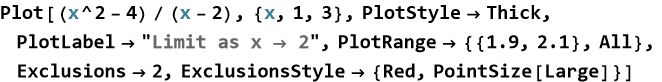
The graph shows a hole at x=2, but the function clearly approaches 4.

Learning to calculate limits efficiently is one of the most practical skills in calculus. The properties we proved earlier do the heavy lifting; our job is to recognize when and how to apply them. In the next sections we will explore one-sided limits, limits at infinity, and continuity—all of which build directly on these calculation techniques.

Exercise 18.2:
a) Evaluate the following limits using direct substitution and the properties of limits:
    1)  
    2)
    3)
b) Evaluate:
    1)
    2)
    Show your algebraic steps clearly.
c) Evaluate .
d) Use Plot to visualize the behavior of near x=3.
e) Look up the description of the WL command Limit. Use this to confirm your answers from a), b), and c).
f) Explain when you can use direct substitution and when you cannot.
g) Why is factoring or rationalizing useful when you get the indeterminate form 0/0.

One-Sided Limits

In the previous section we learned how to calculate many limits using the properties we proved earlier. However, not every limit behaves the same when we approach a point from the left and from the right. Sometimes the function approaches one value from one side and a different value from the other. In these cases, we need the more precise concept of one-sided limits.

Instead of requiring the function to approach the same value from both directions, we can study each direction separately. One-sided limits allow us to examine what happens when we approach a point only from the left or only from the right.

Definition 18.4 Left-Hand Limit: We write and say “the limit as x approaches a from the left is L” if, as x gets closer and closer to a while staying less than a, f(x) gets closer and closer to L.

Definition 18.5 Right-Hand Limit: We write if, as x gets closer and closer to a while staying greater than a, f(x) gets closer and closer to L.

Theorem 18.7: A two-sided limit exists only when both one-sided limits exist and are equal

(18.60)

Proof of Theorem 18.7: We prove this directly, by cases. We prove both directions.

Part 1: Two-sided limit exists ⇒ Both one-sided limits exist and are equal

Assume . Let ε>0 be given. By the definition of the two-sided limit, there exists δ>0 such that if 0<∣x−a∣<δ, then ∣f(x)−L∣<ε. For the left-hand limit, if a−δ<x<a, then 0<∣x−a∣<δ, so ∣f(x)−L∣<ε. Therefore, .

For the right-hand limit, if a<x<a+δ, then 0<∣x−a∣<δ, so ∣f(x)−L∣<ε. Therefore, .

Thus, both one-sided limits exist and equal L.

Part 2: Both one-sided limits exist and are equal ⇒ Two-sided limit exists

Assume and . Let ε>0 be given.

Since the left-hand limit is L, there exists such that if , then ∣f(x)−L∣<ε.

Since the right-hand limit is L, there exists such that if , then ∣f(x)−L∣<ε.

Choose .

Now suppose 0<∣x−a∣<δ. If x<a, then a−δ<x<a, so ∣f(x)−L∣<ε (by the left-hand condition).

If x>a, then a<x<a+δ, so ∣f(x)−L∣<ε (by the right-hand condition).

In either case, ∣f(x)−L∣<ε.Therefore, by the definition of the two-sided limit, . QED

If the left-hand and right-hand limits differ, the two-sided limit does not exist.

For example, we can calculate the one-sided limits of the absolute value function

(18.61)

As x approaches 0 from the left (x→0−), f(x)=−x, so .

As x approaches 0 from the right (x→0+), f(x)=x, so .

Thus, .

Now we consider the piecewise function

(18.62)

Left-hand limit, .

Right-hand limit, .

Since 2≠−2, the two-sided limit does not exist.

We can clearly see one-sided behavior using Wolfram Language.

The graph shows the function approaching 2 from the left and -2 from the right—a classic example of why the two-sided limit fails to exist.

One-sided limits are especially useful when dealing with piecewise functions, physical situations that have a natural direction (such as time approaching a moment from the past), or when analyzing discontinuities.

Mastering one-sided limits gives you a more refined and powerful understanding of how functions behave near critical points.

Exercise 18.3: Begin with Definition 18.4 and copy it into your notebook. Reflect on its meaning for a few minutes. Note any thoughts that come to mind. How would you explain this to someone sitting in front of you. Write this down. Then do this for each definition, theorem, and proof.

Exercise 18.4:
a) Evaluate the following one-sided limits:
    1) .
    2)
    3) Does exist? Explain.


b) Let , find:
    1)


    2)
    3) (if it exists).
c) Consider the function .
    1) Sketch the graph near x=2.
    2) Compute both one-sided limits.
    3) Does the two-sided limit exist? Why or why not?
d) Define the piecewise function from b) in Wolfram Language and plot it.
    1) Use Plot with appropriate options to visualize the behavior near x=3.
    2) Use the Limit command to compute both one-sided limits and the two-sided limit.
    3) Compare the results with your hand calculations.
e) Explain in your own words the difference between a one-sided limit and a two-sided limit.
f) Why is it important to check one-sided limits when working with piecewise functions?

The Squeeze Theorem

We have now seen how to calculate many limits using algebraic properties and direct substitution. But sometimes a function is difficult to simplify directly. In these cases, a powerful tool called the Squeeze Theorem (also known as the Sandwich Theorem) often comes to the rescue. If a function is trapped between two other functions that both approach the same value, then it must also approach that same value. In other words, when a function is squeezed between two others that agree in the limit, it has no choice but to follow them.

Theorem 18.8 The Squeeze Theorem: Suppose that for all x in some open interval around a (except possibly at x=a itself), we have

(18.63)

If

(18.64)

then

(18.65)

In plain language, “If f(x) is “sandwiched” between g(x) and h(x), and both the lower and upper functions approach the same limit L, then f(x) must also approach L.

Imagine three graphs near x=a. The graph of g(x) is below, the graph of h(x) is above, and f(x) is trapped in between. As x approaches a, the lower and upper graphs both get closer and closer to the horizontal line y=L. The trapped function f(x) has nowhere else to go then it must also approach L.

Proof of Theorem 18.8: This is a direct ε-δ proof. Let ε>0 be given (our arbitrary positive tolerance). Since , there exists such that if , then ∣g(x)−L∣<ε. Since , there exists such that if , then ∣h(x)−L∣<ε.

Now choose

(18.66)

Assume 0<∣x−a∣<δ. Then both of the above conditions hold, so, L−ε<g(x)<L+ε and L−ε<h(x)<L+ε, we can combine these inequalities, L−ε<g(x)≤f(x)≤h(x)<L+ε.

Therefore, L−ε<f(x)<L+ε,which is exactly, f(x)−L∣<ε.This is precisely what the definition of the limit requires. Hence, . QED

Use the Squeeze Theorem when you have inequalities that bound your function, the bounding functions have limits that are easy to evaluate, or when direct substitution or algebraic simplification leads to an indeterminate form. The Squeeze Theorem is especially valuable in proving limits involving absolute values, and expressions with square roots.

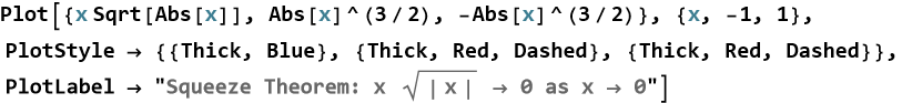
For example, we can evaluate

(18.67)

For all real x, we know that

(18.68)

A better and tighter bound is

(18.69)

When x≥0, , and the expression is positive. When x<0, , and the expression is negative. In both cases, the absolute value satisfies . Therefore, (18.67) is produced.

Now take the limit as x→0

(18.70)

Since is squeezed between two functions that both approach 0, by the Squeeze Theorem

(18.71)

Exercise 18.5: Begin with Theorem 18.8 and copy it into your notebook. Reflect on its meaning for a few minutes. Note any thoughts that come to mind. How would you explain this to someone sitting in front of you. Write this down. Then do this for each theorem and proof.

Trigonometric Limits

We have learned how to calculate many limits using algebraic simplification and the properties of limits. Now we turn our attention to a special and extremely important class of limits involving trigonometric functions. These limits appear again and again in calculus.

Even though sine and cosine oscillate, certain combinations of them have very clean and predictable limiting behavior as the angle approaches zero. Trigonometric limits often rely on the geometric fact that for small angles, the sine of the angle is approximately equal to the angle itself (when measured in radians).

Theorem 18.9:

(18.72)

Proof of Theorem 18.9: This is a geometric proof using the Squeeze theorem. Consider a unit circle. Let θ be a small positive angle in radians. In the unit circle we can compare three lengths where the vertical leg of the small right triangle, sin ⁡θ. The arc length along the circle is θ. The vertical leg of the larger right triangle is tan ⁡θ.

From the geometry, these lengths satisfy, sin⁡ θ<θ<tan ⁡θ=sin ⁡θ/cos⁡ θ. Dividing all parts by the positive number sin ⁡θ, 1<θ/sin θ<1/cos ⁡θ.

Taking reciprocals (and reversing the inequalities), cos ⁡θ<sin⁡ θ/θ<1.

As θ->0+ we know cos⁡θ→1. Therefore, the function sin⁡θ/θ is squeezed between cos ⁡θ and 1, both of which approach 1. By the Sandwich Principle,

(18.73)

A similar argument (using symmetry of the sine function) shows that

(18.74)

Since both one-sided limits are equal, the two-sided limit exists and equals 1

(18.75)

:lim⁡x→0sin⁡xx=1.QED

Theorem 18.10:

(18.76)

Proof of Theorem 18.10: We prove this directly using a trigonometric identity. We begin with the double-angle identity for cosine

(18.77)

Substitute this into the expression

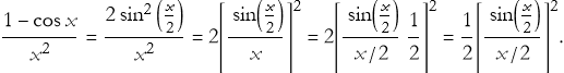
(18.78)

Now take the limit as x→0

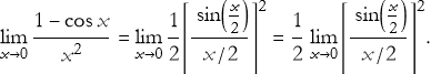
(18.79)

Let u=x/2. As x→0, we also have u→0. Therefore,

(18.80)

(by Theorem 18.9). Thus,

(18.81)

QED

Exercise 18.6: Begin with Theorem 18.9 and copy it into your notebook. Reflect on its meaning for a few minutes. Note any thoughts that come to mind. How would you explain this to someone sitting in front of you. Write this down. Then do this for each theorem and proof.

Exercise 18.7:
a) Evaluate the following limits:
    1) .
    2)
    3) .


b) Evaluate the following limits:
    1)
    2)
    3) .
c) Evaluate the following limits:.
    1)
    2) .
d) Determine whether the following limits exist. If they do, find their value:
    1)
    2)
    3) .
e) Use the Squeeze Theorem to prove .
f) Evaluate:
    1)
    2)

Limits and Infinity

We have learned how to evaluate limits as x approaches a finite number a. But many important situations in physics and mathematics involve behavior as x becomes extremely large (approaching infinity) or as a function grows without bound near a point. These are the realms of limits and infinity.

We can still make precise statements about what happens even when quantities become arbitrarily large or when functions blow up to infinity. In other words, limits give us a rigorous language to describe behavior at infinity and infinite behavior near a point.

For situations where x becomes arbitrarily large we write to mean that as x becomes larger and larger (goes to positive infinity), the value of f(x) gets closer and closer to L.

Similarly, describes behavior as x becomes a very large negative number.

For example

(18.82)

as x->∞, 1/x->0, so

(18.83)

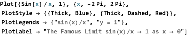
In another example,

(18.84)

even though sin ⁡x oscillates, dividing by larger and larger x forces the expression toward zero.

(18.85)

Sometimes a function grows without bound as x approaches a finite number. We write to mean that as x approaches a, f(x) becomes larger and larger without any upper bound.

For example

(18.86)

This behavior corresponds to a vertical asymptote at x=0.

Wolfram Language makes these behaviors easy to see.

Limits at infinity help us understand long-term behavior—for example, what happens to a population as time goes to infinity, or how an object’s speed approaches a terminal velocity. Infinite limits help us identify vertical asymptotes and singularities in physical models.

Mastering both types of limits gives you a more complete picture of how functions behave across their entire domain, including at the “edges” of reality.

Exercise 18.8:
a) Evaluate .


b) Evaluate the one-sided limits and determine if the two-sided limit exists:
    
    
    
c) Evaluate and .
d) Evaluate and .
e) Evaluate .
f) Use the Squeeze Theorem to prove that the limit .

The Completeness of Real  Numbers

When we work with real numbers, something powerful and often invisible is always at work, the fact that the real line has “no gaps.” No matter how we cut the number line, there is always a number exactly at the cut. This property—called completeness—guarantees that certain sets always have a “highest” or “lowest” point (in a precise sense), even if that point is not obvious at first. This is what allows many important theorems in calculus to be true.

Let S be a non-empty subset of R.

Definition 18.6 Upper Bound:  An upper bound of S is a number M such that ∀(x∈S)x≤M.

Definition 18.7 Supremum: The supremum of S (denoted sup ⁡S) is the smallest upper bound of S.

Definition 18.8 Lower Bound: A lower bound of S is a number m such that ∀(x∈S)x≥m.  

Definition 18.9 Infimum: The infimum of S (denoted inf⁡ S) is the greatest lower bound of S.

Definition 18.10 Maximum: If sup ⁡S actually belongs to S, then sup ⁡S is called the maximum of S.

Definition 18.11 Minimum: If inf ⁡S actually belongs to S, then inf ⁡S is called the minimum of S.

Axiom 18.1 Least Upper Bound Property (Completeness Axiom): Every non-empty subset of real numbers that is bounded above has a least upper bound in R.

For example, if we define a closed interval S=[2,5] then sup S=5 (which is also the maximum), inf S=2 (the minimum).

For an open interval, S=(0,1), then sup S=1, and inf S=0. Neither supremum nor infimum is in S, but they still exist in R.

For the set S={1,1/2,1/3,1/4,… }, then sup S=1 and inf S=0.

For the set , then and . (This shows why must exist in the reals—the set is bounded above but has no rational maximum.)

The idea of a supremum is closely related to limits. When we say we mean L is like a “least upper bound” for the values that f(x) eventually stays below (or above). Completeness guarantees that such limiting values exist when the function behaves nicely. The completeness property fails for the rational numbers. For example, the set of rationals whose square is less than 2 is bounded above but has no rational least upper bound. This is one reason we work with the real numbers in calculus.

Exercise 18.9: Begin with Definition 18.6 and copy it into your notebook. Reflect on its meaning for a few minutes. Note any thoughts that come to mind. How would you explain this to someone sitting in front of you. Write this down. Then do this for each definition and axiom.

Exercise 18.10:
a) For each set ( S ), find sup⁡ S, inf S, and state whether each is attained (i.e., is a maximum or minimum).
    1) S=[-4,7]
    2) S=(0,5)
    3) S={1,2,3,4,5}




b) Consider the intervals and .  
    1) Find , , , and .
    2) Explain why even though the sets are different.
c) Give an example of each of the following (or explain why none exists):
    1) A set S that is bounded above but has no maximum.
    2) A set T that is bounded below but has no minimum.
    3) A set U that is bounded but has neither a maximum nor a minimum.
d) Let .
    1) Is S bounded above? If so, what is an upper bound?
    2) Does S have a least upper bound in the rational numbers?
    3) What is sup S in the real numbers? Explain why this shows the importance of completeness.
e) Let f(x)=(3x+2)/(x+5) for x≥0.
    1) Show that the set S={f(x)∣x≥0} is bounded above by 3.
    2) Find sup S.
    3) How does this relate to ?
f) Let f be continuous on [0, 3] with f(0)=−1 and f(3)=5. Let k=2.
    1) Explain why the set T={x∈[0,3]∣f(x)≤2} is non-empty and bounded above.
    2) Why must supT exist?
    3) Discuss why you expect f(sup ⁡T)=2.

Continuity via Limits

Imagine tracing the graph of a function with your pencil. If you can do so without ever lifting the pencil—without any sudden jumps, holes, or breaks—the function is behaving nicely at every point. Its output values change in a predictable way as the input changes, whenever you are close to a particular input value a, the function’s outputs stay close to a single specific number. This predictable, unbroken behavior is called continuity.

Definition 18.12 Continuity at a Point: A function f is continuous at x=a if the following three conditions hold:

f(a) is defined (a belongs to the domain of f).

The limit exists.

.

If any of these fails, we say f is discontinuous at x=a.

We can also speak of one-sided continuity. A function that is continuous from the right at a has . A function that is continuous from the left at a has .

Definition 18.13 Continuity on an Interval: A function is continuous on an open interval (c, d) if it is continuous at every point inside it. It is continuous on a closed interval [c, d] if it is continuous on (c, d) and also continuous from the right at c and from the left at d.

When the “no breaks” rule is violated, the failure usually falls into one of three categories:

1. Definition 18.14 Removable Discontinuity: The limit exists, but: the function is either undefined at a or does not equal the limit value. The graph has a “hole” at a. If we redefine the function at x=a  by setting f(a)=L, the new function becomes continuous at a. The discontinuity can literally be removed by changing (or adding) a single point.

For example,

(18.87)

where

(18.88)

but f(2) is undefined. Defining f(2)=4 removes the discontinuity.

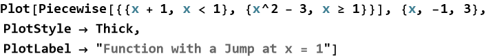
2. Definition 18.15 Jump Discontinuity: Both one-sided limits exist, but they are not equal. The graph “jumps” from one height to another.

For example,

(18.89)

where we have the left limit = 1, and the right limit = –1.

3. Definition 18.16: Infinite (or Essential) Discontinuity (an example of a pole): At least one one-sided limit is +∞  or −∞  (vertical asymptote).

For example

(18.90)

this clearly trends towards ±∞ as x tends towards 3, the sign depends on which direction the limits approaches from.

Theorem 18.11 Intermediate Value Theorem (IVT): If f is continuous on the closed interval [a, b] and k is any number between f(a) and f(b), then there is at least one c between a and b such that f(c)=k.

Proof of Theorem 18.11: This is a proof by contradiction. Define the set

(18.91)

S is non-empty because a∈S (since f(a)<k). We also can say that S is bounded above by b, so by the least upper bound property of the real numbers, S has a supremum c=sup S. Clearly a≤c≤b.

We will show that f(c)=k.

Step 1: Prove f(c)≤k (by contradiction)

Suppose f(c)>k. Since f is continuous at c, there exists δ>0 such that if ∣x−c∣<δ, then ∣f(x)−f(c)∣<(f(c)−k)/2. This implies f(x)>k for all x in (c−δ,c+δ)∩[a,b].  But then all points in (c−δ,c] would be greater than any element of S, contradicting that c=sup S. Therefore, f(c)≤k.

Step 2: Prove f(c)≥k (by contradiction)

Suppose f(c)<k. Again, by continuity, there exists δ>0 such that if |x−c∣<δ, then f(x)<k.  Now consider any point x with c<x<min⁡(b,c+δ). For such x, f(x)<k, so x could be added to S, meaning points larger than c are in S. This contradicts c=sup S. Therefore, f(c)≥k.

From Steps 1 and 2 we conclude that f(c)=k.  Moreover, c≠a (because f(a)<k) and c≠b (because f(b)>k), so c∈(a,b). QED

Algebra of Continuous Functions:
Sums, differences, products, quotients (where defined), and compositions of continuous functions are continuous.

Theorem 18.12: Let f and g be functions from R to R. If f is continuous at a point a and g is continuous at a, then their sum h(x)=f(x)+g(x) is also continuous at a.

Proof of Theorem 18.13: This is a direct proof. Since f is continuous at a, we know that . Since g is continuous at a, we know that . We must show that . By the limit law for sums, if both limits exist, then . Substituting the known limits . This is exactly the third condition needed for h(x)=f(x)+g(x) to be continuous at a. (The first two conditions—h(a) defined and the limit existing—are automatically satisfied.) Therefore, h is continuous at a. QED

Exercise 18.11: Begin with Definition 18.12 and copy it into your notebook. Reflect on its meaning for a few minutes. Note any thoughts that come to mind. How would you explain this to someone sitting in front of you. Write this down. Then do this for each definition, theorem, and proof.

Exercise 18.10:
a) Prove Theorem 18.13: Let f and g be functions from R to R. If f is continuous at a point a and g is continuous at a, then their sum h(x)=f(x)-g(x) is also continuous at a.




b) Prove Theorem 18.14: Let f and g be functions from R to R. If f is continuous at a point a and g is continuous at a, then their sum h(x)=f(x)g(x) is also continuous at a.
c) Prove Theorem 18.14: Let f and g be functions from R to R. If f is continuous at a point a and g is continuous at a, then their sum h(x)=f(x)/g(x) is also continuous at a.
d) Consider the function .
    1) Check whether f is continuous at x=2 by verifying the three conditions.
    2) If it is discontinuous, classify the type of discontinuity.
e) Let for x≠3.
    1) Find .
    2) Is f continuous at x=3? If not, how can you redefine f(3) to make it continuous?
    3)  What type of discontinuity does the original function have?
f) Consider the piecewise function .
    1) Compute both one-sided limits at x=0.
    2) Is f continuous at x=0?
    3) Classify the discontinuity and sketch the graph near x=0.
g) For the function f(x)=1/(x-2)
    1) Find and .
.    2) Is f continuous at x=2?
    3) What type of discontinuity does it have? Describe the graph near x=2.
h) Let .
    1) Show that f is continuous on [0, 2].
    2) Evaluate f(0) and f(2).
    3) Use the Intermediate Value Theorem to prove that there is at least one root between 0 and 2.
i) Explain the three conditions for continuity at a point in your own words.
j) Give one example each of a removable discontinuity, a jump discontinuity, and an infinite discontinuity.
k) Why is the Intermediate Value Theorem important?

Summary

Write a summary of this chapter.

For Further Study

Donald W. Hight, (1977), A Concept of Limits, Prentice-Hall Inc, reprinted by Dover Publications in 1977. A very nice survey of the idea and properties of limits, focusing on sequences and series.

O. Lexton Buchanan, Jr., (1974), Limits A Transition to Calculus, Houghton-Mifflin Company. This text also focuses on sequences and series.

George B. Thomas, Jr., (1965), Continuity, Addison-Wesley Publishing Company, Inc. This book is drawn from a set of lectures at MIT on elementary calculus from an advanced point of view.

Introduction to Limits – Khan Academy
A clear, beginner-friendly start to what limits mean intuitively and from graphs/tables. Perfect entry point.

Limits, L’Hôpital’s Rule, and Epsilon-Delta Definitions (Chapter 7, Essence of Calculus) – 3Blue1Brown
Stunning visual intuition for limits as the “core idea” of calculus. Highly recommended for building deep understanding.

Limits and Continuity – Krista King Math
Solid walkthrough of techniques for finding limits and classifying continuity (removable, jump, infinite discontinuities).

Calculus 1 Lecture 1.4: Continuity of Functions – Professor Leonard
In-depth lecture style (full class feel) covering continuity definitions, types of discontinuities, and the Intermediate Value Theorem. Excellent for thorough learners.

Limits and Continuity | Calculus – Nerdstudy
Straightforward explanation tying limits directly to continuity at a point, with good graphical examples.