Lesson 16 Coordinate Geometry with an Introduction to Vectors and Matrices

“Each problem that I solved became a rule, which served afterwards to solve other problems.” René Descartes

“We think basis-free, we write basis-free, but when the chips are down we close the office door and compute with matrices like fury.” Paul Halmos

Introduction

We have spent many lessons building intuition through geometry and trigonometry. We drew rays, identified similar triangles, and used angles to understand how lenses form images. Now we take a decisive step forward: we will learn how to place that geometry on a precise numerical foundation.

In this lesson we enter the world of coordinate geometry. By assigning numbers to points in space, we gain the ability to calculate distances, describe lines and planes with equations, and turn geometric ideas into algebraic tools we can manipulate. This marriage of geometry and algebra is one of the most powerful inventions in the history of science. It allows us to move seamlessly from pictures we can draw to equations we can solve.

We begin by exploring the Euclidean plane and Euclidean space , the natural settings for most of classical physics. We will examine Gauss’s famous experiment with light rays and curved surfaces, then introduce the Cartesian coordinate system (that we have been using for many lessons) that Descartes gave us—the rectangular grid that makes calculation straightforward.

From there we study the basic objects that live in these spaces: points, lines, and planes. We will prove the distance formula, derive the midpoint formula, and work with the concept of slope. These ideas lead naturally to the equation of a straight line and to applications such as the path of a projectile, the electric field around a point charge, and the distance between planets. We will even look at a simple model of a particle confined in a box.

Next we turn to vectors. We begin by thinking of vectors as arrows that carry both magnitude and direction. We will define vector arithmetic in Euclidean spaces and carefully prove fundamental properties such as the commutativity of scalar multiplication and the distributivity of the scalar product over vector addition. This prepares us for the more abstract idea of a vector space and for the important physical vectors we meet in mechanics and electromagnetism: position, velocity, acceleration, and force vectors. We will also visualize magnetic field lines around a current-carrying wire and inside a solenoid.

Because we have already worked with ray tracing in geometric optics, we will return to optical systems and see how coordinate geometry and vectors help us describe the behavior of light more precisely.

Finally, we introduce matrices. At first they may look like mere arrays of numbers, but they are far more powerful. Matrices let us perform operations on many quantities at once, approximate slopes, represent geometric transformations, and describe the rotation of rigid bodies. We will explore matrix operations, see how matrices can represent changes of coordinates, and use the Wolfram Language to visualize how a matrix transforms points in space. Along the way we will solve systems of linear equations and prove several important matrix properties.

By the end of this lesson you will have a solid toolkit and you will be able to move freely between geometric pictures and algebraic descriptions, handle vectors with confidence, and begin using matrices to organize and transform information. These tools are not abstract—they are the everyday language of theoretical physics. They will let you describe motion, fields, forces, and optical systems with clarity and precision.

As Descartes observed, once we learn to turn the world into coordinates and equations, each problem we solve becomes a rule that helps us solve the next. Welcome to coordinate geometry and the beginning of vector and matrix methods. Let us begin.

The Euclidean Plane

Before we introduce coordinates, we need to be clear about the space we are working in. In this lesson we will spend most of our time in the Euclidean plane, denoted . What do we mean by the Euclidean plane? It is the familiar flat surface you can draw on a piece of paper, extending infinitely in all directions, with no curvature and no boundaries. In this plane, the geometry you learned in Lesson 12, parallel lines never meet, the sum of the angles in any triangle is exactly 180°, and the shortest path between two points is a straight line segment.

We call this geometry Euclidean in honor of the ancient Greek mathematician Euclid, who organized these ideas into a logical system more than two thousand years ago. The Euclidean plane is the simplest and most natural setting for most of classical physics. When we describe the motion of a projectile, the electric field around a point charge, or the path of a light ray through thin lenses, we almost always assume the background space is Euclidean.

The Euclidean plane has several key characteristics that we can use. First, it is flat, there is no overall curvature. A triangle drawn anywhere in the plane always has interior angles that add to exactly 180°. Second, iy is homogeneous and isotropic, where the plane looks the same everywhere and in every direction. No point is special, and no direction is preferred. Third, distance is well-defined and the distance between any two points depends only on their positions and follows the familiar Pythagorean theorem once we introduce coordinates. Finally, straight lines are the shortest paths and in Euclidean geometry, the geodesic (shortest path) between two points is always a straight line.

These properties feel obvious because we live in a world that appears locally flat.

Why should we start here? The reason is practical. Almost all the mathematics and physics we will develop in this book—vectors, matrices, mechanics, electromagnetism, and optics—starts from the assumption that we are working in Euclidean space. By making this assumption explicit, we create a solid foundation. Later, when we study general relativity or more advanced differential geometry, we will see what changes when space itself becomes curved. For now, the flat Euclidean plane gives us the cleanest possible arena in which to learn coordinate methods.Think of as an infinite sheet of graph paper with no edges. Every point on this sheet can eventually be labeled with a pair of numbers (its coordinates). Once we have those numbers, we can calculate distances, draw lines, find slopes, and describe physical quantities such as velocity and force with precision.

Terms

Term 16.1 Homogeneous Space: A space in which every point is equivalent—no location is special or preferred.

Term 16.2 Isotropic Space: A space in which every direction is equivalent—no direction is preferred over any other.

Definitions

Definition 16.1 Euclidean Plane (): The infinite, flat, two-dimensional space in which ordinary plane geometry holds. It has no curvature, no boundaries, and extends forever in all directions. Every point in can be uniquely identified once a coordinate system is chosen.

Definition 16.2 Flat Geometry: Geometry in which the sum of the interior angles of any triangle is exactly 180°, parallel lines never meet, and the shortest path between two points is a straight line segment.

Definition 16.3 Geodesic: The shortest path between two points in a given space. In the Euclidean plane , every geodesic is a straight line.

Exercise 16.1: Begin with Definition 16.1 and copy it into your notebook. Reflect on its meaning for a few minutes. Note any thoughts that come to mind. How would you explain this to someone sitting in front of you. Write this down. Then do this for each term and definition.

The Euclidean Space

Having established the Euclidean plane as our flat, two-dimensional stage, we now take one very natural step upward—we move into three-dimensional Euclidean space, denoted .

Imagine taking the infinite flat sheet of the Euclidean plane and adding a third direction perpendicular to it. The result is the familiar space we live in—the space in which we walk, throw balls, build machines, and watch light travel through lenses. is simply the Euclidean plane extended by one extra dimension. It remains perfectly flat, homogeneous, and isotropic, just like , but now every point requires three numbers to specify its location.

In , the same Euclidean rules continue to hold exactly. The sum of the angles in any triangle is still precisely 180°. Parallel lines never meet, no matter how far they are extended. The shortest path between any two points is a straight line segment. Distance between points is given by the three-dimensional version of the Pythagorean theorem.

Most of classical theoretical physics takes place in this three-dimensional Euclidean space. When we describe the trajectory of a projectile, the electric field surrounding a point charge, the motion of a planet around the Sun, the force on a charged particle, or the path of a light ray through an optical system, we almost always assume the background geometry is .

Why do we care about three dimensions? The jump from to s not merely adding one more number. It opens up an enormous range of new physical phenomena. In the plane we could describe motion left and right, forward and backward. In space we can also move up and down. This third direction lets us talk about the full path of a thrown ball (which rises and falls under gravity), the three-dimensional spread of an electric or magnetic field, the orientation and rotation of rigid bodies, and the focusing of light rays by lenses and mirrors in real optical instruments as examples.

We can establish some properties of . Like the Euclidean plane, three-dimensional Euclidean space is flat, having no intrinsic curvature. Triangles, planes, and straight lines behave exactly as our intuition expects. It is homogeneous, where every point looks the same; there is no special location. It is isotropic, where every direction is equivalent; there is no preferred direction in space. It is infinite and unbounded, where it extends forever in all three directions with no edges or boundaries. These properties make an ideal arena for classical mechanics, electromagnetism, and geometric optics.

Definitions

Definition 16.4 Euclidean Space : The infinite, flat, three-dimensional space that extends forever in all directions with no curvature or boundaries. It is the natural generalization of the Euclidean plane obtained by adding a third perpendicular direction. Every point in is specified by three real numbers once a coordinate system is chosen.

Exercise 16.2: Begin with Definition 16.4 and copy it into your notebook. Reflect on its meaning for a few minutes. Note any thoughts that come to mind. How would you explain this to someone sitting in front of you. Write this down.

Gauss’s Experiment

We have described the Euclidean plane and Euclidean space as flat, homogeneous, and isotropic—the natural stage for most classical physics. But how do we know that the physical space around us really behaves like ? One of the earliest and most famous attempts to test this question experimentally was carried out by Carl Friedrich Gauss in the 1820s during his geodetic survey of the Kingdom of Hanover.

Gauss needed accurate maps, so he established a network of triangulation points across the landscape. Among these were three prominent mountain peaks: Hoher Hagen (near Göttingen), Brocken in the Harz Mountains, and Großer Inselsberg in the Thüringer Wald. The straight-line distances between these peaks were enormous—roughly 69 km, 85 km, and 107 km—forming one of the largest triangles ever measured at the time.

Using precise theodolites (angle-measuring instruments) and his own improved heliotrope (a mirror device that reflected sunlight to create bright, visible signals over long distances), Gauss measured the three interior angles of this giant triangle. In perfect Euclidean space , the sum of the angles in any triangle must be exactly 180°.

Gauss’s measurements gave a sum extremely close to 180°—within the limits of error of his instruments. To the accuracy he could achieve, the geometry of the space near the Earth’s surface behaved exactly like Euclidean space.

At first glance, this looks like a direct test of whether physical space is Euclidean. However, the story is a bit more subtle. The lines of sight Gauss measured were light rays traveling through the atmosphere, and the triangle itself lay on (or slightly above) the curved surface of the Earth. Gauss was aware of this and carefully accounted for the known curvature of the Earth’s surface in his calculations.

He was not primarily hunting for evidence of non-Euclidean geometry in the universe at large. Instead, he was performing a practical check on the consistency of his surveying network and exploring how curvature affects large-scale measurements. He even computed the tiny angular discrepancies that would arise from the Earth’s curvature and found them negligible for his purposes.

Still, the experiment remains historically important. It was one of the first serious attempts to use real-world measurements to probe the geometry of the space we inhabit. Gauss himself was deeply interested in the foundations of geometry and privately explored ideas that later became non-Euclidean geometry, though he never published those thoughts for fear of controversy.

Why does this matter for us? Gauss’s experiment reminds us that geometry is not just abstract mathematics—it can be tested against the real world. To the precision available in the 1820s, physical space near Earth is Euclidean. This is why we confidently use as the background for classical mechanics, electromagnetism, and geometric optics.

On much larger scales or in the presence of very strong gravity, general relativity tells us that space-time is curved. But for almost everything we will do in this book—projectile paths, electric fields, ray tracing through lenses, and rigid body rotations—the Euclidean approximation is extraordinarily accurate and far simpler to work with.

Definitions

Definition 16.5 Gauss’s Great Triangle: The large triangulation triangle formed by the mountain peaks Hoher Hagen (near Göttingen), Brocken (Harz Mountains), and Großer Inselsberg (Thüringer Wald), with sides approximately 69 km, 85 km, and 107 km. Gauss measured the interior angles of this triangle in the 1820s.

Definition 16.6 Theodolite: A precise optical instrument used for measuring horizontal and vertical angles between distant points. Gauss used theodolites to determine the angles at each vertex of the great triangle.

Definition 16.7 Heliotrope: An instrument invented by Gauss consisting of a mirror that reflects sunlight to create a bright, visible signal over long distances, allowing accurate sighting between mountain peaks.

Definition 16.8 Lines of Sight: The straight paths traveled by light rays from one mountain peak to another, treated as straight lines in Euclidean space .

Principles

Principle 16.1 Local Euclidean Geometry Principle: .On ordinary human and surveying scales (tens to hundreds of kilometers), physical space near the Earth’s surface behaves locally like flat Euclidean space .

Principle 16.2 Light-Ray-as-Geodesic Principle: In the context of geometric surveying and optics, light rays traveling through the atmosphere are treated as straight-line geodesics in .

Principle 16.3 Gauss’s Caution Principle: Even when privately exploring non-Euclidean ideas, Gauss refrained from publishing them due to fear of philosophical and scientific controversy (a reminder of the importance of rigorous evidence before challenging established views).

Exercise 16.3: Begin with Definition 16.5 and copy it into your notebook. Reflect on its meaning for a few minutes. Note any thoughts that come to mind. How would you explain this to someone sitting in front of you. Write this down.

The Cartesian Coordinate System

Having seen Gauss’s experiment—where precise measurements of angles and distances in real three-dimensional space confirmed that, to high accuracy, we live in Euclidean space —we now need a practical way to attach numbers to every point in that space. The Cartesian coordinate system is the tool that makes this possible. It is the rectangular grid invented by René Descartes that lets us describe any location with a set of numbers and turn geometry into algebra.

In the Cartesian system we choose three straight lines (the axes) that intersect at a single point called the origin. These axes are labeled x, y, and z. Once the origin and the positive directions are fixed, every point P in can be uniquely specified by an ordered triple of real numbers (x, y, z), called the Cartesian coordinates of P.

Orthogonal versus Nonorthogonal Coordinate Systems

The simplest and most useful Cartesian system is orthogonal: the three axes are mutually perpendicular (they meet at right angles). This choice is natural in Euclidean space because perpendicularity preserves the Pythagorean theorem and makes distance calculations clean

(16.1)

Nonorthogonal (oblique) systems are possible—the axes may intersect at angles other than 90°—but they complicate formulas for distance, angles, and areas. In almost all classical physics we therefore use orthogonal axes. The orthogonality assumption is what makes the coordinate system “Cartesian” in the everyday sense.

Right-Handed and Left-Handed Systems

Once the axes are chosen to be orthogonal, we still have a choice of orientation. Imagine pointing the thumb of your right hand along the positive x-axis and the index finger along the positive y-axis. Your middle finger will then point along the positive z-axis. This is the right-handed coordinate system and is the universal convention in physics and engineering.

The opposite choice—where the z-axis points the other way—produces a left-handed system. The two systems are mirror images of each other.

Parity

The difference between right-handed and left-handed systems is an example of parity. A parity transformation is a mirror reflection through a plane (or an inversion through the origin). Under such a reflection, a right-handed coordinate system becomes left-handed, and vice versa.

In physics, parity is important because many fundamental laws (electromagnetism, mechanics, gravity) are unchanged under mirror reflection—they are parity invariant. For most of the work in this book we will adopt the right-handed orthogonal Cartesian system as the standard. It is the convention used in nearly all textbooks and computational software (including Wolfram Language). Once you become comfortable with it, switching to a left-handed system is simply a matter of reversing the direction of one axis.

Why the Cartesian System Is Powerful?

Gauss’s great triangle was measured using angles and distances without coordinates. The Cartesian system lets us translate those same measurements into numbers we can manipulate algebraically. With coordinates we can:compute exact distances instantly, write equations for lines, planes, and trajectories, describe rotations,and prepare the ground for matrices and linear transformations.

In short, the Cartesian coordinate system turns the abstract Euclidean space into a concrete numerical framework. It is the bridge between the geometric pictures we draw and the algebraic calculations we need for theoretical physics.

Definitions

Definition 16.9 Cartesian Coordinate System: A method of assigning an ordered triple of real numbers (x, y, z) to every point in Euclidean space . The numbers represent signed distances from three mutually perpendicular axes that intersect at a chosen origin.

Definition 16.10 Origin: The fixed point where the three coordinate axes intersect. It is usually denoted by the point (0, 0, 0).

Definition 16.11 Coordinate Axes: Three straight lines (the x-axis, y-axis, and z-axis) that pass through the origin and are mutually perpendicular in an orthogonal Cartesian system.

Definition 16.12 Orthogonal (Rectangular) Cartesian System: A coordinate system in which the three axes are pairwise perpendicular (meet at 90° angles). This is the standard Cartesian system used in classical physics.

Definition 16.13 Right-Handed Coordinate System: The conventional orientation in which, if the thumb of the right hand points along the positive x-axis and the index finger along the positive y-axis, the middle finger points along the positive z-axis. This satisfies the right-hand rule.

Definition 16.14 Left-Handed Coordinate System: The mirror-image orientation obtained by reversing the direction of one axis (usually the z-axis). It is the opposite of the right-handed system.

Definition 16.15 Parity Transformation: A mirror reflection through a plane or an inversion through the origin (x,y,z)→(−x,−y,−z). A parity transformation converts a right-handed system into a left-handed one, and vice versa.

Definition 16.16 Cartesian Coordinates of a Point P: The ordered triple (x, y, z) such that x is the signed distance from the y z-plane, y is the signed distance from the x z-plane, and z is the signed distance from the x y-plane.

Principles

Principle 16.4 Right-Hand Rule Convention: In physics and engineering, the positive orientation of the axes is chosen so that the right-hand rule holds. This is the universal standard in textbooks and computational tools.

Principle 16.5 Parity Invariance Principle: Many fundamental laws of classical physics (mechanics, electromagnetism, gravity) are unchanged under parity transformations (mirror reflections). Therefore, the choice between right-handed and left-handed systems is largely a matter of convention.

Principle 16.6 Uniqueness of Representation: Once the origin and the positive directions of the three orthogonal axes are fixed, every point in has a unique set of Cartesian coordinates (x, y, z).

Theorems

Theorem 16.1 Distance Formula in Cartesian Coordinates: The Euclidean distance between two points and in

(16.2)

Proof of Theorem 16.1: We shall produce a direct geometric proof using the Pythagorean theorem. Consider two points and in Euclidean space .

From draw a line parallel to the x-axis to reach the point

.
From (Q), draw a line parallel to the y-axis to reach the point .

Finally, from R draw a line parallel to the z-axis to reach .

These three segments — Q, QR, and —are mutually perpendicular because the coordinate axes are orthogonal. Apply the Pythagorean theorem in stages. First, in the plane parallel to the x y-plane (constant ). The distance from to Q is . The distance from Q to R is. These two segments form a right triangle with hypotenuse from to R. By the Pythagorean theorem

(16.3)

Next, consider the right triangle formed by R and the vertical segment from R to , whose length is ∣z2−z1∣. The line from is the hypotenuse of this larger right triangle. Again apply the Pythagorean theorem

(16.4)

Take the square root. Since distance is positive, we obtain

(16.5)

QED

Exercise 16.4: Begin with Definition 16.9 and copy it into your notebook. Reflect on its meaning for a few minutes. Note any thoughts that come to mind. How would you explain this to someone sitting in front of you. Write this down. Do this for each definition, principle, theorem, and proof.

Exercise 16.5:
a) Plot the following points in a right-handed Cartesian coordinate system and describe their locations relative to the origin and the coordinate planes:
    1)  A(3, 0, 0)
    2) B(0,−4,0)
    3) C(0, 0, 5)
    4) D(2,−3,4)
    For each point, state which coordinate planes it lies on or is closest to.
b) Calculate the straight-line (Euclidean) distance between each pair of points using the distance formula. Show your work.
    1) and
    2) and
    3) The origin (0,0,0) and the point R(5,12,0)
c) Describe the right-hand rule for a Cartesian coordinate system. If you reverse the direction of the z-axis, does the system become right-handed or left-handed? Explain why physics textbooks almost always use the right-handed         convention.
d) Why does using orthogonal (perpendicular) axes make the distance formula simple? Suppose the axes are not perpendicular. What complication would arise when calculating the distance between two points? Give one reason why     we almost always choose orthogonal Cartesian coordinates in classical physics.
e) A projectile is launched from the origin with initial position (0,0,0). After some time it reaches the point (20, 15, 8) meters.
    1) Calculate the straight-line distance from the launch point to this position.
    2) If the motion were confined to the x y-plane (z = 0), what would the distance be?
    3) Explain how the third coordinate (z) changes the physical description compared to a 2D case.
f) You are designing a simple optical system. Place the center of a thin convex lens at the origin (0,0,0). An object is located at (−25, 0, 0) cm and the image forms at (16.7, 0, 0) cm along the optical axis (x-axis).
    1) What are the coordinates of the object and image?
    2) Calculate the object distance and image distance using the distance formula (note that they are simply the absolute differences along the x-axis).
    3) Explain how the Cartesian coordinate system makes it easy to extend this 1D description to full 3D ray tracing in later sections.

Curvilinear Coordinates

Having mastered the Cartesian coordinate system, we can now describe any point in with three numbers (x, y, z). Cartesian coordinates are excellent when the problem has straight lines, rectangular symmetry, or flat boundaries. But nature often presents us with circular, cylindrical, or spherical symmetry. Planets orbit in nearly circular paths, electric fields spread spherically from a point charge, a solenoid produces cylindrical magnetic fields, and a rotating carousel or a lens system has rotational symmetry. In these cases, Cartesian coordinates become awkward—equations get cluttered with square roots and trigonometric functions that do not reflect the underlying symmetry.

Curvilinear coordinates adapt the coordinate grid to the natural shape of the problem. The most useful ones in theoretical physics are polar, cylindrical, and spherical coordinates. Each system still covers the entire Euclidean space
(or for polar coordinates), but uses coordinates that make symmetry obvious and calculations simpler.

An important concept for coordinate systems is that of the distance between nearby point. We call this the length element or line element. In Cartesian coordinates the line element is,

(16.6)

We use the symbol d represents a very small distance.

Polar Coordinates (2D)

In the Euclidean plane a point can have these coordinates (r,θ) and we can see that there is a transformation from polar to Cartesian coordinates

(16.7)

Here r≥0 is the radial distance from the origin, and θ is the angle measured counterclockwise from the positive x-axis (in radians).

The inverse transformation is

(16.8)

We must take care for the correct quadrant.

The length element in polar coordinates

(16.9)

Cylindrical Coordinates (3D)

Cylindrical coordinates extend polar coordinates by adding the Cartesian z-coordinate

where

(16.10)

Here φ is the azimuthal angle. We can also state that , z∈(−∞,∞) and , φ∈[0,2π).

We can write the length element

(16.11)

This is perfect for problems with cylindrical symmetry (pipes, wires, solenoids, coaxial cables).

Spherical Coordinates (3D)

Spherical coordinates are the most natural choice when a problem has spherical symmetry.

(16.12)

Here r≥0 is the radial distance from the origin, θ∈[0,π] is the polar angle (from the positive z-axis), and φ∈[0,2π) is the azimuthal angle.

The length element is then

(16.13)

This form appears a lot in gravitational fields and electromagnetic fields.

Definitions

Definition 16.17 Curvilinear Coordinates: Any coordinate system in which the coordinate surfaces (constant-coordinate surfaces) are curved rather than flat planes. They are chosen to match the natural symmetry of a problem, making equations simpler and more intuitive.

Definition 16.18 Polar Coordinates (2D): A coordinate system in the Euclidean plane where a point is specified by the radial distance r≥0 from the origin and the angle θ.

Definition 16.19 Cylindrical Coordinates (3D): An extension of polar coordinates into by adding the Cartesian height z.

Definition 16.20 Spherical Coordinates (3D): A coordinate system ideally suited for spherical symmetry. mHere a point is specifie by its radial distance from the origin, r>0, the angle θ is the angle measured from the positive z axis to the radial line connecting to the point—called the polar angle, and φ is the angle around the z axis on the x y plane—called the azimuthal angle.
Definition 16.21 Length Element (Line Element) (ds): An extremely small distance between two nearby points in a given coordinate system.

Definition 16.22 Coordinate Transformation: The set of equations that convert coordinates from one system (e.g., curvilinear) to another (usually Cartesian).

Principles

Principle 16.7 Symmetry Principle: Choose a coordinate system whose coordinate surfaces match the natural symmetry of the problem at hand (circular → polar/cylindrical, spherical → spherical). This greatly simplifies the mathematical description.

Principle 16.8 Orthogonality of Curvilinear Systems: The standard polar, cylindrical, and spherical coordinate systems are orthogonal, that is the coordinate curves (lines of constant other coordinates) intersect at right angles. This preserves many of the nice properties of Cartesian coordinates while adapting to curvature.

Principle 16.9 Length Element Invariance: The distance ds between two points is independent of the coordinate system chosen. The expression for changes form, but its value remains the same.

Principle 16.10 The Right-Hand Rule Convention: In cylindrical and spherical coordinates, the azimuthal angle φ increases in the right-handed sense around the z-axis (counterclockwise when viewed from above the positive z-axis).

Principle 16.11 Coordinate Choice Principle: There is no single “best” coordinate system. The skillful physicist chooses the system that makes the symmetry of the problem manifest, thereby simplifying the resulting differential equations.

Principle 16.12 Equivalence of Descriptions: All correctly formulated physical laws must give the same physical predictions regardless of the coordinate system used. The length element ensures that distances and geometries remain consistent across systems.

Exercise 16.6: Begin with Definition 16.17 and copy it into your notebook. Reflect on its meaning for a few minutes. Note any thoughts that come to mind. How would you explain this to someone sitting in front of you. Write this down. Do this for each definition, and principle.

Exercise 16.7:
a) A point in the plane has Cartesian coordinates (x,y)=(−3,4).
    1) Convert this point to polar coordinates (r,θ). Give r exactly and θ in radians (principal value, −π<θ≤π).
    2) Verify your answer by converting back to Cartesian coordinates.
    4) Write the length element ds in polar coordinates and use it to find the arc length along a circle of radius r=5 units from θ=0 to θ=π/2.
b) A point has cylindrical coordinates (r,φ,z)=(5,π/3,4).
    1) Convert this point to Cartesian coordinates (x, y, z).
    2) Convert it to spherical coordinates (r,θ,φ).
c) A point lies at spherical coordinates (r,θ,φ)=(6,π/3,π/4).
    1) Convert to Cartesian coordinates.
    2) Convert to cylindrical coordinates.
    3) At this point, a small displacement has dr=0.1, dθ=0.05 rad, and dφ=0.1 rad. Use the spherical length element to estimate the total distance moved.

Subspaces: Points, Lines, and Planes

Having learned both Cartesian and curvilinear coordinate systems, we can now describe the simplest geometric objects that live inside Euclidean space , points, lines, and planes. These are the fundamental “subspaces” we will use constantly in physics.

Points

A point is the simplest object in space. In Cartesian coordinates it is specified by an ordered triple (x, y, z). In cylindrical coordinates it is (r,φ,z), and in spherical coordinates it is (r,θ,φ). No matter which system we choose, a single point is completely determined by its coordinates.

Lines

A straight line in is the shortest path between two points. It extends infinitely in both directions.

Parametric Equations

A parametric representation of a line expresses each coordinate x, y, and z as a function of a single independent parameter, usually called t (which can be thought of as a “time” or “progress” variable along the line).

If a line passes through point and has the direction arrow d=⟨a,b,c⟩, then any point on the line can be written as

(16.14)

(16.15)

(16.16)

where t is a real parameter (−∞<t<∞).

If

(16.17)

then we classify the equations (16.14), (16.15), and (16.16) as symmetric equations.

In polar or cylindrical coordinates, lines not passing through the axis become more complicated, which is why we usually use Cartesian coordinates for lines.

Planes

A plane is a flat two-dimensional surface extending infinitely. It is the 3D analogue of a straight line in 2D. The general equation of a plane is

(16.18)

where a, b, and c are fixed numbers that tell us the direction that is perpendicular to the plane (in other words the a line dropped from the triple to the plane will be perpendicular) and d is a constant. If the plane passes through point then

(16.19)

this is called the point-normal form (normal because that is the same as perpendicular).

In curvilinear coordinates these objects can look more complicated (a straight line not along a coordinate axis becomes a curve in polar coordinates), which is why we often switch back to Cartesian coordinates when working with lines and planes.

Definitions

Definition 16.23 Subspace: A geometric object (point, line, plane, etc.) that is contained within Euclidean space and satisfies the same basic geometric rules as the larger space.

Definition 16.23 Point: The simplest geometric object in space. In Cartesian coordinates, a point is specified by an ordered triple of real numbers (x,y,z). It has position but no size or direction.

Definition 16.24 Straight Line: The unique shortest path between two distinct points in that extends infinitely in both directions.

Definition 16.25 Plane: A flat, two-dimensional surface that extends infinitely in all directions within .

Definition 16.26 Parametric Equations of a Line: A set of three equations that describe every point on a line using a single parameter t

(16.20)

where is a known point on the line and a, b, and c are fixed numbers that determine the direction of the line.

Definition 16.27 Symmetric Equations of a Line: When a, b, and c are all nonzero we have an alternative description of a line

(16.21)

Definition 16.28 General Equation of a Plane:  Any plane in can be written in the form

(16.22)

where a, b, and c are not all zero.

Definition 16.29 Perpendicular Direction to a Plane (Normal Direction): The unique direction (up to sign) that makes a right angle with every line lying in the plane. In the equation (16.22), the numbers a, b, and c together specify this perpendicular direction.

Exercise 16.8: Begin with Definition 16.23 and copy it into your notebook. Reflect on its meaning for a few minutes. Note any thoughts that come to mind. How would you explain this to someone sitting in front of you. Write this down. Do this for each definition, and principle.

Exercise 16.9:
a) Plot or describe the location of the following points in a right-handed Cartesian coordinate system:
    1) A(4, 0, 0)
    2) B(0,−3,0)
    3) C(0, 0, 5)
    4) D(−2,3,−4)
For each point, state which coordinate plane(s) it lies on or is closest to, and give a brief physical interpretation (e.g., position of an object).
b) A straight line passes through the point (2, 1, 3) and has direction numbers a=3, b=−1, c=2.
    1) Write the parametric equations of the line.
    2) Find the points on the line when t=0, t=1, and t=−2.
    3) Does the point (8,−1,7) lie on this line? Show your reasoning.


c) A line passes through the points and .
    1)  Find the symmetric equations of the line.
    2)  Write the parametric equations using the same direction numbers.
    3) Find where this line intersects the x y-plane (where z=0).
d) A plane passes through the points A(1, 0, 0)), (B(0, 2, 0)), and (C(0, 0, 3).
    1) Find the general equation of the plane in the form a x+b y+c z=d.
    2)  Write the equation in point-normal form using point A.
    3) Does the point (1, 1, 1) lie on this plane? Verify your answer.
e) A light ray travels in a straight line through space. It passes through the point (0, 0, 0) and the point (3, 6, 2).
    1) Write parametric equations for the path of the ray.
    2) Find the point on the ray when the parameter t=4.
    3) Suppose this ray strikes a plane given by the equation x+y+z=12. Find the coordinates of the intersection point.
f) Try to follow the following.
    1) Explain why every straight line in can be described using parametric equations.
    2) Why is the general equation of a plane a x+b y+c z=d useful in physics? Give at least two physical examples.
    3)  Compare the advantages of parametric equations for lines versus the general equation for planes. When would you choose one form over the other?

Midpoint

One of the most useful simple calculations we can perform with points in Euclidean space is finding the point that lies exactly halfway between two given points—we call this point the midpoint.

Theorem 16.2 The Midpoint Formula: Let and be any two points in . The midpoint M of the line segment joining them has coordinates

(16.23)

In other words, each coordinate of the midpoint is simply the average of the corresponding coordinates of the two endpoints.

Proof of the Midpoint Formula: We produce a direct proof. Let M have the proposed coordinates

(16.24)

We must show two things:

M lies on the line passing through and .

The distance from to M equals the distance from M to .

Step 1: Show M lies on the line.

Using the parametric equations of the line through and , any point on the line can be written

(16.25)

Set ,

(16.26)

(16.27)

(16.27)

Thus, when , the parametric equations give exactly the point M. Therefore M lies on the line.

Step 2: Show the distances are equal.

Compute the distance from   to M

(16.29)

The distance from M to   yields exactly the same expression (just swap the indices). Therefore

(16.30)

Since M lies on the line and is equidistant from the two endpoints, it is the midpoint of the segment . QED

The midpoint formula is remarkably simple because each coordinate is treated independently. This independence comes from the orthogonal nature of the Cartesian coordinate system. The formula works equally well in two dimensions (just drop the z-coordinate) and extends naturally to any number of dimensions.

Exercise 16.10:
a) Find the midpoint of the line segment joining each pair of points:
    1) A(2, 4, 1) and B(8, 10, 7)
    2) C(−3,0,5) and D(5,0,−1)


    3) The origin (0,0,0) and the point E(6,−8,4)
b) The midpoint of a line segment is M(4,−1,3). One endpoint is . Find the coordinates of the other endpoint .


c) A straight line passes through points A(1, 2, 3) and B(7, 8, 9).
    1)  Find the midpoint of segment AB.
    2)  Find the point that is one-quarter of the way from A to B.
    3) Find the point that is three-quarters of the way from A to B.

Slope

In the previous section we learned how to find the midpoint of a line segment—the point exactly halfway between two given points. Now we introduce another fundamental idea in coordinate geometry, the rate measuring how fast something rises or falls, what we call: the slope of a line or curve.

Slope of a Straight Line

Consider two distinct points and in the Euclidean plane . The slope m of the straight line passing through these points is defined as the ratio of the vertical change (rise) to the horizontal change (run)

(16.31)

provided (the line is not vertical). If we introduce new notation,

(16.32)

This does not mean Δ times y, instead it means the change in y. So we can rewrite (16.31)

(16.33)

A positive slope means the line rises as we move to the right. A negative slope means the line falls as we move to the right. A slope of zero means the line is horizontal. A vertical line has undefined slope (division by zero).

The slope is constant for any straight line—no matter which two points you choose on the line, the value of m is the same.

Slope of a Function at a Point

For a curved graph given by a function y=f(x), the idea of slope becomes more subtle. At any specific point on the curve, we can draw a tangent line—the straight line that just touches the curve at that point and has the same direction as the curve.

The slope of the function at a point x=a is defined as the slope of this tangent line at that point. It tells us the instantaneous rate of change of the function at x=a.

Although we will study this idea more carefully when we reach calculus, we can already understand it geometrically in coordinate space where the slope at a point measures how steeply the graph is rising or falling right at that location.

Why Slope Matters in Physics

Slope connects geometry directly to rates of change:

The slope of a position-time graph gives velocity.

The slope of a velocity-time graph gives acceleration.

In optics, the slope of a ray path helps determine angles of incidence and refraction.

In electric circuits, the slope of a voltage-current graph gives resistance.

Understanding slope in coordinate space gives you an intuitive foundation for the more advanced concept of derivatives you will meet later.

The slope of a straight line is constant. The slope of a curve changes from point to point — and that changing slope is what makes curves interesting and powerful in theoretical physics.

Definitions

Definition 16.30 Slope (of a straight line): The ratio of the vertical change (rise) to the horizontal change (run) between any two distinct points on the line

(16.34)

(provided ).

Definition 16.31 Slope of a Function at a Point: The slope of the tangent line to the graph of the function y=f(x) at a specific point x=a. It represents the instantaneous rate of change of the function at that point.

Definition 16.32 Tangent Line: The straight line that touches a curve at a given point and has the same direction (slope) as the curve at that exact location.

Definition 16.33 Rise: The vertical change

(16.35)

Definition 16.33 Run: The horizontal change

(16.36)

Axioms

Axiom 16.1 Uniqueness of Slope for Straight Lines: Any straight line (that is not vertical) has exactly one constant slope value, independent of which pair of points on the line is chosen.

Axiom 16.2 Sign Interpretation Axiom: The sign of the slope determines the direction of the line:

Positive slope → line rises from left to right.

Negative slope → line falls from left to right.

Zero slope → line is horizontal.

Undefined slope → line is vertical.

Principles

Principle 16.13 Constant Slope Principle: The slope of a straight line is the same between any two points on that line.

Principle 16.14 Local Linearity Principle: Near any point on a smooth curve, the graph behaves approximately like a straight line (its tangent line). The slope of this tangent line gives the best linear approximation to the curve at that point.

Principle 16.15 Coordinate Independence of Geometric Meaning: While the numerical value of the slope depends on the coordinate system, the concepts of steepness and direction are geometric properties independent of the specific axes chosen.

Exercise 16.11: Begin with Definition 16.30 and copy it into your notebook. Reflect on its meaning for a few minutes. Note any thoughts that come to mind. How would you explain this to someone sitting in front of you. Write this down. Do this for each definition, axiom, and principle.

Exercise 16.12:
a) Find the slope of the straight line passing through each pair of points:
    1) (2, 3) and (5,9)
    2) (-1,4) and (5,9)


    3) The origin (0,0) and the point (4, 0)
    4) (2,5) and (2,8)
    For each, state whether the line rises, falls, is horizontal, or is vertical.
b) A position-versus-time graph for a moving object is a straight line with slope m=3.5 m/s.
    1) What physical quantity does this slope represent?
    2)  If the slope were −2  m/s, what would that mean physically?
    3) What would a slope of zero indicate?


c) Find the slope of each of the following lines given in standard form:
    1)  3x−4y=12
    2)  y=−2x+5
    3) x=7  (vertical line)
    4) y=4 (horizontal line)
d) The graph of a function y=f(x) passes through the point (2, 8) and has a tangent line at that point with slope m=−3.
    1) Write the equation of the tangent line at x=2.
    2) Use the tangent line to approximate the value of the function at x=2.2.
    3) Is the function increasing or decreasing at x=2? How steeply?
e) A light ray travels in a straight line from point (0, 0) to point (10, 4).
    1) Calculate the slope of the ray.
    2) If this ray strikes a mirror lying along the line y=6, find the coordinates of the impact point.
    3) Explain what the slope tells you physically about the direction of the light ray.
f) Explain in your own words the difference between the slope of a straight line and the slope of a curve at a single point.
g) Why can a vertical line not have a defined slope?
h) Give two physical situations (different from those in previous exercises) where knowing the slope of a line or tangent is important in theoretical physics.

Approximation of Slope

In the previous section we learned how to find the exact slope of a straight line and how to interpret the slope of a curve at a single point as the slope of its tangent line. Now we ask a very practical question, “How can we estimate the slope of a curve at a particular point when we do not yet know how to calculate the exact tangent line?”

The Basic Idea

Consider the graph of a function y=f(x). Pick a point P on the curve where x=a. To estimate the slope at P, choose another nearby point Q on the same curve where x=a+Δ x  and Δ x is a small number.

Draw the straight line that connects P and Q. The slope of this connecting line gives a good approximation to the true slope of the curve at point P. As we make the second point Q closer and closer to P (that is, as we make Δ x smaller and smaller), this connecting line gets closer and closer to the true tangent line at P. Therefore, its slope becomes a better and better estimate of the actual slope we are looking for.

The Difference Quotient

The slope of the line connecting P and Q is given by the expression

(16.37)

This quantity is called the difference quotient. It represents the average rate of change of the function between x=a.

Example

Let’s take the function and estimate the slope at x=2. If Δ x=0.1, then

(16.38)

If Δ x=0.01, then

(16.39)

If Δ x=0.001, then

(16.40)

You can see that as Δ x gets smaller, the approximation gets closer to 4, which is the true slope at that point.

Why This Idea Is Important?

This method of using two nearby points to estimate the slope at a single point is one of the central ideas that leads into calculus.

The smaller we make the step Δ x, the better the approximation becomes. You can approximate the slope of a curve at any point by calculating the slope of a straight line connecting two very close points on that curve.

Definitions

Definition 16.34 Approximation of Slope: A method of estimating the slope of a curve at a point by using the slope of a straight line connecting two nearby points on the curve.

Definition 16.35 Secant Line: A straight line that connects two distinct points on a curve. Its slope gives an approximation to the true slope of the curve at a chosen point.

Definition 16.36 Difference Quotient: The expression

(16.41)

that gives the slope of the secant line between the points where x=a and x=a+Δ x.

Definition 16.37 Average Rate of Change: The slope of a secant line over an interval. It measures how much the function changes on average between two points.

Definition 16.38 Instantaneous Rate of Change: The slope of the tangent line at a single point. It measures the exact rate of change of the function at that precise location.

Principles

Principle 16.16 Secant-to-Tangent Principle: As the second point Q moves closer and closer to point P (i.e., as Δ x becomes smaller and smaller), the secant line approaches the tangent line, and its slope becomes a better and better approximation to the true slope at P.

Principle 16.17 Improvement with Smaller Steps: The smaller the step size Δ x, the more accurate the slope approximation becomes.

Principle 16.18 Local Linearity Principle: Near any point on a smooth curve, the graph behaves approximately like a straight line. The slope of this approximating line gives useful information about the local behavior of the function.

Principle 16.19 Physical Interpretation Principle: The slope approximation (the difference quotient) often represents a physically meaningful average rate—such as average velocity over a short time interval—and that approaches the instantaneous rate as the interval shrinks.

Exercise 16.13: Begin with Definition 16.34 and copy it into your notebook. Reflect on its meaning for a few minutes. Note any thoughts that come to mind. How would you explain this to someone sitting in front of you. Write this down. Do this for each definition,  and principle.

Exercise 16.14:
a) Consider the function .
    1) Calculate the slope of the secant line between x=3 and x=3+Δ x when Δ x=0.1.
    2) Repeat for Δ x=0.01 and Δ x=0.001.


    3) What value does the secant slope appear to approach as Δ x gets smaller?
b) For the function at the point x=2.
    1) Compute the difference quotient for Δ x = 0.5, 0.1, and 0.01.
    2) Describe what happens to the approximation as Δ x decreases.
    3) Based on the pattern, guess the true slope (tangent slope) at x=2.


c) The position of a particle is given by meters, where t is time in seconds.
    1)  Find the average velocity between t=1 sec and t=1.2 sec.
    2)  Find the average velocity between t=1 sec and t=1.01 sec.
    3) Explain how these calculations approximate the instantaneous velocity at t=1 sec.
d) The graph of a function passes through the point (4, 10). A nearby point on the curve is (4.2, 10.88).
    1) Calculate the slope of the secant line between these two points.
    2) If you move the second point to (4.05, 10.4025), recalculate the secant slope.
    3) Which approximation is better, and why?
e) For f(x)=sin  x at x=π/2.
    1) Compute the secant slope using Δ x=0.1.
    2) Compute it again using Δ x=0.01.
    3) The true slope (tangent slope) at this point should be 0. Explain why your approximations are approaching this value.
f) In your own words, explain why making Δ x smaller improves the slope approximation.
g) What happens if Δ x is too large? Give a physical example where a large step size would give a poor approximation.
h) Why is this method of approximation important in physics.

The Equation of the Line

We now know how to find or approximate the slope of a line or curve. But how do we describe the entire line using an equation? How can we write down a rule that tells us exactly where every point on that line lies?

The basic idea is simple, if we know one point on the line and we know its slope, we can write an equation that gives the y-coordinate for any x-coordinate on that line. This turns the geometric picture of a straight line into a compact algebraic description.

The Main Idea

Suppose we have a straight line that passes through a known point and has a constant slope m. For any other point (x, y) on the same line, the slope between these two points must equal m as seen in the previous sections. We modify the equation

(16.42)

This is the heart of the matter. Rearranging gives us a useful equation for the line.

Point-Slope Form

Multiplying both sides by   produces the point-slope form of the equation of a line

(16.43)

This form is especially convenient because it directly uses a known point and the slope.

Slope-Intercept Form

If the line crosses the y-axis at the point (0, b), then we can write the equation as

(16.44)

where b is the y-intercept. This is called the slope-intercept form. It is often the simplest form when we want to see both the slope and where the line crosses the y-axis at a glance.

Example

A line passes through the point (2, 3) with slope m=4.Using point-slope form

(16.45)

This is also the slope-intercept form, with y-intercept −5.

Once we have the equation of a line, we can do the following

Find any point on the line instantly,

Determine where it intersects other lines or planes,

Describe the path of a light ray, a particle moving with constant velocity, or the boundary of a region.

In physics, the equation of a line lets us turn geometric intuition (“a straight path”) into precise calculations needed for trajectories, optical rays, and many other situations.

The transition from knowing the slope and a point to writing the full equation is one of the most useful skills in coordinate geometry. It connects the visual picture of a line directly to the algebra we need for real calculations.

Definitions

Definition 16.39 Equation of a Line: An algebraic rule that describes all points (x, y) lying on a straight line in the plane. It allows us to find any point on the line or determine whether a given point lies on it.

Definition 16.40 Point-Slope Form: The equation of a line that passes through a known point is

Definition 16.41 Slope-Intercept Form: The equation of a line written as y=m x+b where m is the slope and b is the y-intercept (the value of y when x=0).

Definition 16.42 General Form of a Line: The equation a x+b y+c=0, where a, b and c are constants (not both a and b are not zero).

Axioms

Axiom 16.3 Uniqueness Axiom: Given a point and a slope (or two distinct points), there exists exactly one straight line passing through them in the Euclidean plane.

Axiom 16.4 Consistency Axiom: Any correctly written equation of a line must give the same slope and pass through the same points regardless of the form used (point-slope, slope-intercept, or general).

Principles

Principle 16.20 Coordinate Independence Principle: The geometric properties of a line (its direction and position) do not depend on the particular form of its equation, although different forms are useful for different purposes.

Principle 16.21 Conversion Principle: Any form of the equation of a line can be converted into any other form using algebraic rearrangement.

Exercise 16.15: Begin with Definition 16.39 and copy it into your notebook. Reflect on its meaning for a few minutes. Note any thoughts that come to mind. How would you explain this to someone sitting in front of you. Write this down. Do this for each definition,  axiom, and principle.

Exercise 16.16:
a) A straight line passes through the point (3, 2) with slope m=4.
    1) Write the equation of the line in point-slope form.
    2) Convert it to slope-intercept form.


    3)  Find the point on the line where x=0.
b) Find the equation of the straight line passing through the points A(1, 4) and B(5, 12).
    1) First find the slope..
    2) Write the equation in point-slope form using point A.
    3) Convert the result to slope-intercept form.


c) Convert the equation y=−3x+7 to the general form.
    1)  Write the general form.
    2)  Verify that the points (0, 7) and (2, 1) both satisfy your equation.
    3) What is the slope of this line?
d) A light ray starts at the point (0, 0) and passes through the point (6, 4)..
    1) Write the equation of the ray in slope-intercept form.
    2) Using that equation, find where the ray intersects the line y=8.
    3) Interpret the slope physically: what does it tell you about the direction of the light ray?
e) The equation of a line is 2x+5y=20.
    1) Convert it to slope-intercept form and identify the slope and y-intercept.
    2) Find two different points that lie on this line.
    3) Write the point-slope form using one of the points you found.
f)  Explain in your own words why knowing the equation of a line is more powerful than just knowing its slope and one point.
g) A particle moves along a straight line with constant velocity. Its position at time t=0 is (2, 1) and its velocity components are and (units per second). Write the parametric         equations and the Cartesian equation of its path.
h) Why is the equation of a line especially useful when working with optical rays or trajectories in physics?

The Path of a Projectile

We now know how to write the equation of a straight line. But many real motions in nature are not straight. One of the most common and important curved paths is the trajectory of a thrown or launched object—a projectile.

Imagine throwing a ball. While it flies through the air, two things happen at the same time. It moves horizontally (sideways) at a roughly constant speed (ignoring air resistance). It moves vertically, pulled downward by gravity, so its vertical speed changes constantly.

The actual path you see is the combination of these two independent motions. The surprising result is that this combined path is a smooth curve called a parabola.

Let’s describe the motion using coordinates. Suppose we launch the projectile from the origin (0, 0) with initial horizontal speed and initial vertical speed .

We can write the horizontal motion (no acceleration)

(16.46)

We can write the vertical motion (constant downward acceleration g

(16.47)

To find the path—that is, the relationship between y and x—we eliminate the time t.

From the horizontal equation, solve for t

(16.48)

Substitute this into the vertical equation

(16.49)

Simplifying gives the equation of the trajectory

(16.50)

This is the equation of a parabola. Notice how it extends the idea of the equation of a line, instead of a simple linear relationship, we now have a quadratic term that creates the characteristic curved shape.

Even though the path is curved, we can still describe it with a single equation in x and y. This is the power of coordinate geometry—we turn a complicated real-world motion into something we can analyze algebraically.

The horizontal motion is uniform (like a straight line with constant slope in the absence of gravity), but gravity bends the path downward. The resulting parabola is one of the most common curves in classical physics—appearing in the motion of cannonballs, baseballs, rockets (before engines cut off), and even electrons in certain fields.

By writing the equation of the path, we can answer practical questions: Where will it land? What is its maximum height? How does changing the launch angle affect the range?

This section shows how the tools we have built—coordinates, slope, and the equation of a line—naturally extend to describe curved motion. The same ideas will help us understand many other physical phenomena in later lessons.

Exercise 16.17:
a) A projectile is launched from the origin with initial horizontal velocity m/s and initial vertical velocity m/s. Take g=10   downward.
    1) Write the equation of the trajectory y as a function of x.
    2) What is the shape of the path?


    3)  At what horizontal distance does the projectile hit the ground again.
b) Using the same launch conditions as Exercise 16.17 a).
    1) Find the time when the projectile reaches its maximum height.
    2) Use the trajectory equation to find the maximum height.
    3) At what horizontal distance does this maximum height occur?


c) The trajectory of a projectile is given by the equation .
    1)  What was the initial vertical velocity component if m/s?
    2)  What is the maximum height reached?
    3)  Where does the projectile land?
d)  Explain in your own words why the path of a projectile is a parabola even though gravity pulls only vertically.
e)  How does the horizontal motion being uniform (constant velocity) lead to the parabolic shape when combined with vertical acceleration?
f)  Why is the equation of the trajectory useful even if we ignore air resistance?

A Particle in a Box

We have just seen how coordinate geometry lets us describe the curved path of a projectile with a single equation. Now we turn to a simpler but very important situation, where a particle moving back and forth between two walls. This model helps us understand confined motion and appears in many areas of physics, from classical mechanics to quantum theory.

Imagine a tiny ball sliding without friction on a straight track. The track has hard walls at both ends. The ball moves at constant speed until it hits a wall, then bounces back with the same speed in the opposite direction. It keeps repeating this motion forever.

The key question is, “How can we describe where the particle is at any moment using coordinates?”

Place the box along the x-axis with walls at x=0 and x=L, where L is the length of the box. The particle moves only along this line, so its position at any time is given by a single number x(t), where 0≤x(t)≤L.

Assume the particle starts at position with initial velocity (positive if moving to the right). Between collisions, it moves with constant speed, so its position changes linearly with time—just like the horizontal part of the projectile motion we saw earlier.

When it hits a wall, its velocity reverses direction (the sign of v flips), but the speed stays the same. This creates a repeating back-and-forth motion.

One useful way to think about the position is to “unfold” the box, where we imagine the particle continuing in a straight line through an infinite series of identical boxes placed side by side. In this unfolded picture the motion is simple uniform motion, but when we fold it back into the real box, the path appears as a zigzag.

For small times before any collision, the position is simply

(16.51)

After hitting a wall, the velocity changes sign, and the expression updates accordingly. The motion is piecewise linear—straight-line segments connected at the walls.

Even though the motion looks simple, the “particle in a box” is one of the most important model systems in physics. It helps us understand

Confined motion and bouncing.

Standing waves.

Basic behavior of electrons in wires, atoms in crystals, or gas molecules in a container.

By using coordinate geometry, we can write down exact expressions for the particle’s position at any time, calculate how often it hits each wall, and determine its average speed. This gives us a concrete example of how to move from a physical picture (“a ball bouncing between walls”) to precise mathematical descriptions using the tools of coordinates and equations.

The particle in a box shows us that even very simple setups can lead to rich and useful mathematics—a pattern we will see again and again in theoretical physics.

Exercise 16.18:
a) A particle moves back and forth inside a one-dimensional box of length L=4 m. It starts at x=1 m with velocity +3  m/s (to the right).
    1) Write the position for the time interval before it first hits a wall.
    2) At what time does it first hit a wall?


    3) What is its velocity immediately after that collision?
b) A particle in a box of length L=10 m moves with constant speed v=5 m/s.
    1) How long does it take to go from one wall to the opposite wall?
    2) What is the total time for one complete round trip (from left wall to right wall and back)?
    3)  Sketch the position versus time for the first two round trips.


c) A particle starts at the center of a box (x=L/2) with initial velocity .
    1)  Write the position as a function of time until it hits the first wall.
    2)  Describe qualitatively what the motion looks like over a long time.
    3)   How does changing the starting position affect the motion?
d) A particle bounces back and forth in a box of length L with constant speed v.
    1) What is its average velocity over one full round trip?
    2) What is its average speed over one full round trip?
    3) Why are the two answers different?
e) Consider the particle in a box as moving along a straight line that “reflects” at the walls.
    1) How is this motion similar to the horizontal part of a projectile’s path?
    2) How is it different?
    3) Write a short paragraph explaining how the equation of a line helps us understand the particle’s motion between collisions.
f)  Explain in your own words why the “particle in a box” is a useful model in physics.
g)  What changes if the particle loses a tiny amount of speed each time it hits a wall?
h)  Why do physicists often study this simple system before moving to more complicated real-world situations?

Conic Sections

We have seen how a particle bouncing between the walls of a box follows straight-line segments, and how a projectile follows a smooth curved path called a parabola. Nature produces many other beautiful curved paths. Planets move in closed curves around the Sun, comets swing in open curves, and mirrors and lenses are often shaped in specific curves to focus light. All of these important curves belong to one remarkable family.

Imagine taking a right circular cone (like an ice-cream cone) and slicing it with a flat plane at different angles. Depending on the angle of the cut, you get different elegant curves. These curves—called conic sections—appear throughout physics because they naturally arise from simple physical laws, especially those involving inverse-square forces like gravity.

There is also a beautiful geometric way to define these curves using a point called a focus and a line called a directrix. This focus-directrix definition turns out to be extremely useful in astronomy and optics.

Suppose you have a curve such that the sum of the distances from any point on the curve to two fixed points (called foci) is always the same constant. This curve is an ellipse. An ellipse is a closed, oval-shaped curve. The Sun sits at one focus of Earth’s elliptical orbit. The other focus is empty. This remarkable property—that the total distance to the two foci is constant—leads directly to Kepler’s laws of planetary motion.

Here is the equation of an ellipse

(16.52)

The two foci are located at (±c,0) where .

The directrices can be found using the eccentricity , then the directrices are the vertical lines at x=±a/ε.

Kepler’s First Law: Planets move in elliptical orbits with the Sun at one focus.

This single geometric fact, discovered by Kepler and later explained by Newton using gravity, is one of the great triumphs of theoretical physics.

Now imagine a curve where the difference of the distances from any point on the curve to two fixed foci is constant. This curve is a hyperbola. It has two separate branches that open outward.

The equation of a hyperbola is

(16.53)

Hyperbolas appear in the paths of comets that pass the Sun once and then fly off into space, and in certain optical systems and relativity.

We already met the parabola in projectile motion. A parabola can be defined as the set of all points that are the same distance from a fixed point (the focus) as they are from a fixed line (the directrix).

The equation of a parabola is

(16.54)

The focus is at (0,p) and the directrix is y=-p.

This focus-directrix property explains why parabolic mirrors and satellite dishes work so well, we have rays coming in parallel to the axis reflect through the focus (or vice versa).

This beautiful family of curves arises naturally from geometry and appears again and again in physics because the inverse-square law of gravity and electrostatics produces exactly these shapes as orbits and field lines.

From the bouncing particle in a box (straight lines) to projectiles (parabolas) to planets (ellipses), coordinate geometry lets us write precise equations for all these paths. Understanding conic sections gives you a powerful toolkit for describing motion under central forces — whether you are studying gravity, electricity, or optics.

These curves show us once again how simple geometric ideas, when combined with coordinates, reveal the hidden order in the physical world.

Definitions

Definition 16.43 Conic Section: A curve obtained by slicing a right circular cone with a plane at different angles, or equivalently, a curve defined using a focus and a directrix.

Definition 16.44 Ellipse: A closed, oval-shaped curve such that the sum of the distances from any point on the curve to two fixed points (the foci) is constant.

Definition 16.45 Hyperbola: A curve with two separate branches such that the difference of the distances from any point on the curve to two fixed foci is constant.

Definition 16.46 Parabola: A curve consisting of all points that are the same distance from a fixed point (the focus) as from a fixed line (the directrix).

Definition 16.47 Focus (Foci): A special point (or two points) used in the geometric definition of a conic section. For an ellipse and hyperbola there are two foci; for a parabola there is one.

Definition 16.48 Directrix: A fixed line used in the definition of a conic section. For any point on the curve, the distance to the focus and to the directrix are related in a specific way.

Definition 16.49 Eccentricity (ε): A number ε that classifies the type of conic section:

    ε<1 for an ellipse, ε=1 for a parabola, and ε>1 for a hyperbola.

Axioms

Axiom 16.5 Focus-Directrix Definition: Every conic section can be defined as the set of points satisfying a specific distance relationship between a focus and a directrix (with eccentricity ε).

Axiom 16.6 Cone-Slicing Property: All conic sections (ellipse, parabola, hyperbola) can be generated by cutting a right circular cone with a plane at different angles.

Principles

Principle 16.22 Unified Geometric Principle: All conic sections arise from the same geometric idea—a relationship between distances to a focus (or foci) and a directrix—with the value of the eccentricity determining the specific shape.

Principle 16.23 Symmetry Principle: Conic sections possess natural symmetry (reflection symmetry across their axes), which makes their equations simpler and their physical behavior more predictable.

Principle 16.24 Kepler’s First Law Principle: Planets move in elliptical orbits with the Sun at one focus. This is a direct consequence of the geometry of the ellipse and Newton’s law of gravity.

Theorems

Theorem 16.3 Standard Equation of an Ellipse:

(16.55)

Foci are located at (±c,0), where .

Proof of Theorem 16.3: This is a direct proof. Let the two foci be and , where c>0. Let the constant sum of distances be 2 a, where a>c.

For any point P(x, y) on the ellipse, we have

(16.56)

Using the distance formula

(16.57)

Move one radical to the other side

(16.58)

Square both sides

(16.59)

Expand both sides,

(16.60)

Subtract ,

(16.61)

Add 2 c x to both sides

(16.62)

Divide by 4,

(16.63)

Isolate the remaining square root

(16.64)

Divide both sides by a

(16.65)

This tells us that a>0. Square both sides again,

(16.66)

Cancel -2 c x,

(16.67)

Rearrange

(16.68)

Factor this

(16.69)

We can write ,

(16.70)

Divide by

(16.71)

This is the standard equation of the ellipse centered at the origin with major axis along the x-axis. QED

Theorem 16.4 Standard Equation of a Hyperbola:

(16.72)

Foci at (±c,0), where and the eccentricity is ε=c/a<1

Proof of Theorem 16.4: This is a direct proof. Place the two foci at and , where c>a>0. For any point P on the hyperbola,

(16.73)

We will consider the right branch, where

(16.74)

(the left branch is symmetric).

So we have

(16.75)

Isolate one square root

(16.76)

Square both sides

(16.77)

Expanding and simplifying

(16.78)

Cancel , , and

(16.79)

Add 2 c x to both sides

(16.80)

Divide by 4

(16.81)

Isolate the remaining square root

(16.82)

Divide by a

(16.83)

Square both sides again

(16.84)

Expand left side

(16.85)

Cancel −2 c x

(16.86)

Rearrange

(16.87)

Factor

(16.88)

Now define (note because c>a)

(16.89)

Multiply both sides by −1

(16.90)

Divide through by

(16.91)

This is the standard equation of the hyperbola (for the case opening left and right). QED

Theorem 16.5 Standard Equation of a Parabola:

(16.92)

The focus is at (0,p) and the directrix is y=-p.

Proof of Theorem 16.5: This is a direct proof. Place the focus at the point F(0, p) and the directrix as the horizontal line y=−p, where p>0.

Let P(x, y) be any point on the parabola. By definition, the distance from P to the focus is the distance from P to the directrix. Using the distance formula the distance from P(x, y) to the focus  is

(16.93)

The distance from P(x, y) to the directrix is y=-p, this gives us a vertical distance of

(16.94)

So the defining equation is

(16.95)

Eliminate the absolute value and square both sides. Since distances are positive, we can square both sides directly (this removes the square root and the absolute value)

(16.96)

Expand both sides

(16.97)

Subtract from both sides

(16.98)

Add 2 p y to both sides

(16.99)

Divide both sides by 4 p (since p>0)

(16.100)

This is the standard equation of a parabola that opens upward with vertex at the origin (0,0).

Exercise 16.19: Begin with Definition 16.43 and copy it into your notebook. Reflect on its meaning for a few minutes. Note any thoughts that come to mind. How would you explain this to someone sitting in front of you. Write this down. Do this for each definition,  axiom, principle, and theorem.

Exercise 16.20:
a) The equation of an ellipse is .
    1) Identify a and b.
    2) Find the coordinates of the two foci.


    3) Calculate the eccentricity.
b) A planet moves in an elliptical orbit with the Sun at one focus. The semi-major axis is a=4 AU and the eccentricity is ε=0.2.
    1) Calculate the distance from the center to each focus.
    2) What is the minimum and maximum distance from the planet to the Sun?
    3)  Why is this consistent with Kepler’s First Law?


c) The equation of a hyperbola is  
    1) Identify a and b.
    2) Find the coordinates of the two foci.


    3) Calculate the eccentricity.
d) A parabola has focus at (0, 3) and directrix y=−3.
    1) Write the standard equation of this parabola.
    2) Find the vertex.
    3) Sketch the parabola and label the focus and directrix.
e) A projectile is launched from the origin with initial horizontal velocity 12 m/s and initial vertical velocity 16 m/s. Take g=10 .
    1) Write the equation of the trajectory y as a function of x.
    2) What is the maximum height reached?
    3) How far horizontally does it travel before hitting the ground again?
f)  Explain in your own words the unified focus-directrix definition that connects the ellipse, hyperbola, and parabola.
g)  Why do conic sections appear so frequently in physics (give at least two examples)?
h)  How does the equation of a parabola you derived for projectile motion connect to the geometric focus-directrix definition?

Canonical Forms

We have now seen how the beautiful family of conic sections—ellipses, hyperbolas, and parabolas—can be described by simple equations. But in real problems we often start with a more general equation that mixes , (x y), , and linear terms. How can we tell what kind of curve it really represents? The answer is to transform the equation into one of its standard or canonical forms.

Any second-degree equation in two variables can be rewritten, by rotating and shifting the coordinate axes, into one of nine especially simple forms. These nine forms are called the canonical forms of conic sections (including some cases where the geometric figure collapses or breaks down into something simpler, we call such cases degenerate). Once the equation is in canonical form, the geometric nature of the curve becomes obvious at a glance.

The process of transforming a general second-degree equation into one of these nine canonical forms is called reducing the equation to canonical form. It uses two kinds of coordinate transformations:

Rotation of the axes (to eliminate the x y term)

Translation of the origin (to eliminate the linear terms)

After these transformations, the equation simplifies dramatically and reveals exactly what kind of curve we are dealing with.

Here are the nine possible canonical forms and what they represent geometrically

Ellipse  , this forms a closed oval curve.

Imaginary Ellipse,  , no real points exist—the curve is imaginary.

A Single Point (A degenerate ellipse),  , the curve collapses to a single point at the origin.

Hyperbola, , two separate branches opening left and right (or up and down).

Pair of Intersecting Lines (degenerate hyperbola),  , factors into two lines crossing at the origin.

Parabola, , the familiar U-shaped (or inverted U-shaped) curve we saw in projectile motion.

Pair of Parallel Lines, , produces two distinct parallel straight lines.

Pair of Imaginary Parallel Lines, , there are no real points—the lines are imaginary.

Pair of Coincident Lines (a Double Line), =0, produces a single straight line counted twice

By reducing a general second-degree equation to one of these nine canonical forms, we immediately know what geometric object we are dealing with—without having to plot hundreds of points. This technique is extremely useful in theoretical physics because many physical laws (gravitational fields, electric potential, optical surfaces, etc.) lead to second-degree equations. Once we have the canonical form, we can recognize ellipses (planetary orbits), parabolas (projectile paths and mirrors), hyperbolas (some comet trajectories), or even degenerate cases (pairs of lines representing boundaries or nodal lines).

The process of reduction relies on two simple coordinate transformations: rotating the axes to remove the mixed x y term, then shifting the origin to remove the linear terms. After these steps, the equation becomes one of the nine clean forms above.

Mastering canonical forms gives you a powerful diagnostic tool where you can look at any second-degree equation and immediately understand the shape it describes.

Coordinate Transformations

We have seen how powerful it is to reduce a complicated second-degree equation to one of the nine canonical forms. But how do we actually do that? The secret lies in a very useful technique where we change the coordinate system itself to make the equation simpler.

Sometimes the coordinate axes we are using are not aligned with the natural symmetry of the curve. The equation looks messy with extra mixed terms like x y. The solution is to move or rotate the axes so that the curve lines up nicely with the new axes. When we do this, many of the complicated terms disappear, and the equation becomes one of the clean canonical forms we saw earlier.

There are two main kinds of coordinate transformations we use: Translation (shifting the origin) and rotation (turning the axes).

The simplest transformation is to slide the origin to a new location without changing the direction of the axes, this is translation (as we saw in Lesson 12).

Suppose we move the origin from (0, 0) to a new point (h, k). If a point has old coordinates (x, y), its new coordinates (x', y') relative to the shifted origin are

(16.101)

Or, solving for the new coordinates

(16.102)

We shift the origin to the center (or vertex) of the curve. This usually eliminates the linear terms (x and y) and makes the equation cleaner.

Sometimes the axes are tilted relative to the curve. We can rotate the entire coordinate system by an angle θ. If a point has old coordinates has old coordinates (x, y), its new coordinates (x', y') after rotating the axes counterclockwise by angle θ

(16.103)

These are the rotation formulas. They allow us to eliminate the troublesome x y term in a general second-degree equation.

We rotate the axes until they align with the natural axes of symmetry of the curve (the major and minor axes of an ellipse, the transverse axis of a hyperbola, etc.). This removes the cross term x y.

In practice, we often do both. We first rotate the axes to eliminate the x y term. Then translate the origin to eliminate the linear terms.

After these two transformations, any second-degree equation reduces to one of the nine canonical forms we studied in the previous section. This process is what allows us to recognize whether an equation represents an ellipse, hyperbola, parabola, or one of the degenerate cases (pair of lines, single point, etc.).

Being able to change coordinate systems is an essential skill in theoretical physics. It lets us

Simplify complicated equations,

Reveal hidden symmetries,

Choose the most coordinate system for a problem,

Understand the true geometric nature of a curve or surface.

Whether you are analyzing planetary orbits, designing optical systems, or studying electric fields, the ability to transform coordinates gives you powerful control over the mathematics.

Mastering translation and rotation of axes completes the basic toolkit of coordinate geometry. You can now take almost any second-degree equation, transform the coordinates appropriately, and immediately recognize what kind of curve it represents.

Definitions

Definition 16.50 Canonical Form: One of the nine especially simple standard equations that a general second-degree equation can be transformed into by rotating and shifting the coordinate axes.

Definition 16.51 Degenerate Case: A situation in which a conic section collapses or breaks down into a simpler geometric object (a point, a pair of lines, or nothing real).

Definition 16.52 Reduction to Canonical Form: The process of transforming a general second-degree equation into one of the nine canonical forms by using coordinate transformations (rotation and translation).

Definition 16.53 Coordinate Transformation: A change of the coordinate system (by moving or rotating the axes) that leaves the geometric object unchanged but simplifies its equation.

Definition 16.54 Translation of Axes: Shifting the origin to a new point (h,k) without changing the direction of the axes.

Definition 16.55 Rotation of Axes: Turning the coordinate axes by an angle θ around the origin.

Axioms

Axiom 16.7 Existence of Canonical Form: Every general second-degree equation in two variables can be reduced to one of the nine canonical forms by a suitable combination of rotation and translation of axes.

Axiom 16.8 Uniqueness of Reduced Form: After reduction, the canonical form of a given equation is unique up to the orientation and position of the axes.

Principles

Principle 16.25 Simplification Principle: By choosing a coordinate system aligned with the natural symmetry of the curve (through rotation and translation), complicated terms like the x y term and linear terms can be eliminated, revealing the true geometric nature of the equation.

Principle 16.26 Diagnostic Power Principle: Once an equation is reduced to canonical form, its geometric type (ellipse, hyperbola, parabola, or degenerate case) becomes immediately obvious without plotting points.

Principle 16.27 Coordinate Freedom Principle: The geometric properties of a curve do not depend on the choice of coordinate system. We are free to choose the most convenient coordinates (by translation and rotation) to simplify calculations.

Exercise 16.21: Begin with Definition 16.50 and copy it into your notebook. Reflect on its meaning for a few minutes. Note any thoughts that come to mind. How would you explain this to someone sitting in front of you. Write this down. Do this for each definition,  axiom, and principle.

Exercise 16.22:
a) Identify each of the following equations as one of the nine canonical forms and state what geometric object it represents:
    1)  
    2)
    3)
    4)
    5)
b) The equation represents a circle.
    1) Complete the square to rewrite it in a translated coordinate system
    2) What are the coordinates of the center in the original system?
    3) What is the radius?
c) The equation contains a cross term.
    1) Explain why rotating the axes would help simplify this equation.
    2) What is the goal of the rotation?
    3) After rotation, what kind of conic section do you expect this to become?.
d) Reduce the equation to canonical form by completing the square or using appropriate transformations. Identify the resulting curve.
e) Classify each of the following as a degenerate or non-degenerate case and explain what geometric object it represents:
    1)
    2)
    3)  
    4)
f)  You are given the general second-degree equation .
    1) What is the first transformation you would apply if b≠0?
    2) What is the second transformation you would apply afterward?
    3)  Why is this two-step process so useful in theoretical physics?
h)  Explain in your own words why reducing an equation to canonical form is powerful.
i) How do translation and rotation of axes help reveal hidden symmetries?
j) Give one physical example where recognizing the canonical form of an equation would be useful.

Matrices

A matrix is a rectangular array of symbols, often these symbols are numbers. Matrices are almost as important to physics as trigonometry—maybe more so. We say that there are M rows and N columns of a matrix. The number of rows and columns form the order of the matrix. We can also call it an M×N matrix. If the matrix is labeled A, then we will have elements labeled by column and row as indices, we will use the convention that columns are represented by superscripts and rows by subscripts, thus the matrix elements are written, , where i=1,…,M and j=1,…,N.

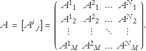
(16.104)

A matrix having one row and N columns, is a row matrix,

(16.105)

A matrix having M rows and a single column, is a column matrix,

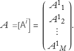
(16.106)

A matrix having the same number of rows and columns is called an N × N square matrix.

If two matrices, say O and P, have the same elements then they are equal and we write O = P.

We can add two matrices by adding their elements,

(16.107)

In order to add matrices the matrices must be of the same order, another word for this is conformable.

We can also subtract two conformable matrices by subtracting their elements,

(16.108)

We can multiply a matrix by a number, say a, by multiplying each element by a,

(16.109)

The number a is often called a scalar for historical reasons (we will see this in later sections. The operation described in Equation (16.109) is called scalar multiplication. The operation of addition, subtraction, and scalar multiplication form the nucleus of matrix arithmetic.

The following rules apply, first addition is commutative,

(16.110)

Addition is associative,

(16.111)

There is an additive identity, in this case it is a matrix all of whose elements are 0, we will label this script 0, ,

(16.112)

This is called the null matrix. The additive identity is then,

(16.113)

There is an additive inverse,

(16.114)

Scalar multiplication is right-distributive,

(16.115)

Scalar multiplication is left-distributive,

(16.116)

If we have a sum, it can be burdensome to write it out every time, instead of writing

(16.117)

we can instead use the upper-case Greek letter sigma, Σ, to denote the sum. Further, below the sigma we will write the summation variable (the variable that informs us as to what we are summing over), and above the sigma we will place the maximum m value of the summation variable. We will write Equation (16.117) this way,

(16.118)

This is called the summation notation, and it is used throughout mathematics and science.

Given two matrices, R and S, where R is an M ×N matrix and S is an N × T matrix the matrix product of the two is

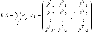
(16.119)

where i=1,…,M, j=1,…N, and k=1,…,T. Where the elements are a set of sums of products,

(16.120)

Assuming all matrices are conformable, then the matrix product is left- and right-distributive and associative

(16.121)

(16.122)

(16.123)

In general, the matrix product is not commutative. In general, O P=, does not imply that either O= or that P=. In general, A B=A C does not imply that B=C.

We now introduce five important kinds of matrices. A square matrix with all off-diagonal elements zero, and all diagonal elements non-zero is called a diagonal matrix. A diagonal matrix whose diagonal elements are all 1, is called the identity matrix, and is denoted I. A square matrix whose elements satisfy the condition , is called an upper triangular matrix. A square matrix whose elements satisfy the condition , is called a lower triangular matrix. Another way of defining a diagonal matrix is that it is both upper and lower triangular.

If O P=I=P O, then P is the inverse matrix of O, . We also note that . Similarly . In general, for a 2 × 2 matrix

(16.124)

A matrix that is the interchange of rows and columns of another matrix is the transpose of that other matrix. We denote this with a T superscript,

(16.125)

The following rules hold.

(16.126)

(16.127)

(16.128)

(16.129)

A matrix equal to its transpose is called symmetric, . A matrix equal to its negative transpose is called skew-symmetric, .

Definitions

Definition 16.56 Matrix: A rectangular array of symbols (usually numbers) arranged in rows and columns.

Definition 16.57 Order of a Matrix: If a matrix has M rows and N columns, it is called an M × N matrix.

Definition 16.58 Element: An individual entry in the matrix, denoted , where superscript i is the row index and subscript j is the column index.

Definition 16.59 Row Matrix: A matrix with one row and N columns.

Definition 16.60 Column Matrix: A matrix with M rows and one column.

Definition 16.61 Square Matrix: A matrix with the same number of rows and columns (N × N).

Definition 16.62 Equal Matrices: Two matrices are equal if they have the same order and all corresponding elements are identical.

Definition 16.63 Conformable Matrices: Matrices that have compatible dimensions for addition or multiplication.

Definition 16.64 Identity Matrix: A square diagonal matrix with 1’s on the main diagonal and 0’s elsewhere, denoted I.

Definition 16.65 Transpose: The matrix obtained by interchanging rows and columns of the original matrix, denoted .

Definition 16.66 Symmetric Matrix: A square matrix equal to its own transpose ().

Definition 16.67 Skew-Symmetric Matrix: A square matrix equal to the negative of its transpose ().

Axioms

Axiom 16.9 Equality Axiom: Two matrices are equal only if they have the same order and every corresponding element is equal.

Axiom 16.10 Addition Axiom: Matrices can be added only if they are conformable (same order).

Axiom 16.11 Multiplication Axiom: Matrix multiplication is defined only when the number of columns of the first matrix equals the number of rows of the second matrix.

Principles

Principle 16.28 Non-Commutativity of Matrix Multiplication: In general, matrix multiplication is not commutative, O P≠P O.
.

Theorems

Theorem 16.6 Commutativity of Addition: Matrix addition is commutative: O+P=P+O.

Proof of Theorem 16.6: This will be a direct proof. Let O and P be two conformable matrices (same order) with elements and , where i=1,…,M and j=1,…,N. By the definition of matrix addition, the (i,j)-th element of the sum O+P is .Similarly, the (i,j)-th element of the sum P+O is. Since the addition of real numbers (scalars) is commutative, for any real numbers a and b we have a+b=b+a.

Applying this to the corresponding elements, we obtain for every pair of indices i and j.  Because every element of O+P equals the corresponding element of P+O, the two matrices are identical, O+P=P+O. QED

Theorem 16.7 Associativity of Addition: Matrix addition is associative, (O+P)+Q=O+(P+Q).

Theorem 16.8 Distributivity of Scalar Multiplication: Scalar multiplication distributes over matrix addition, right-handed a(O+P)=a O+a P and left-handed (a + b)O=a O+b O.

Proof of Theorem 16.8: This will be a direct proof. Let the elements of the matrices be denoted and , where i=1,…,M and j=1,…,N.

We have the left-hand side: a(O+P). First, the (i,j)-th element of the sum O+P is . Now multiply by the scalar a, .

Then we have the right-hand side, a O+a P. the (i,j)-th element of a O is , and the (i,j)-th element of a P is .

Therefore, the (i,j)-th element of a O+a P is .

Since multiplication by a scalar distributes over addition of real numbers, we have for every pair of indices i and j.

Because every corresponding element is equal, the two matrices are identical a(O+P)=a O+a P. QED

Theorem 16.9 Existence of Additive Identity: There exists a null (zero) matrix 0 such that P+0=P.

Proof of Theorem 16.9: This is a direct proof. Define the zero matrix 0 of order M×N as the matrix whose every element is zero

(16.130)

That is, every element   for  i=1,…,M and j=1,…,N. By the definition of matrix addition, the (i,j)-th element of P+0 is . Since this holds for every element  (i,j), we have P+0=P. Thus, the zero matrix 0 acts as the additive identity for matrices of the same order. QED

Theorem 16.10 Uniqueness of Additive Inverse: For any matrix P, there is exactly one matrix Q such that P+Q=0, where 0  is the zero matrix. This unique matrix Q is called the additive inverse of P, and we denote it by −P.

Proof of Theorem 16.10: This is a direct proof. We already know that −P (the matrix whose elements are the negatives of those of P) satisfies

(16.131)

Now suppose there exists another matrix Q that also satisfies

(16.132)

We must show that Q=−P.

Add −P to both sides of equation (16.132)

(16.133)

Using the associativity of matrix addition and the property of the zero matrix on the right side

(16.134)

From equation (16.131), we know P +(-P)=, so we can also write the left side as

(16.135)

Thus Q=−P. Therefore, any matrix that acts as an additive inverse of P must be identical to −P. The additive inverse is unique. QED

Exercise 16.23: Begin with Definition 16.56 and copy it into your notebook. Reflect on its meaning for a few minutes. Note any thoughts that come to mind. How would you explain this to someone sitting in front of you. Write this down. Do this for each definition,  axiom, principle, theorem, and proof.

Exercise 16.24:
a) A matrix A is given by
        
    1)  What is the order of this matrix?
    2) Write the element and .
    3) Is this a row matrix, column matrix, or neither?
b) Let
        
        
    1) Compute O+P.
    2) Compute O−P.
    3) Verify that (O+P)+Q=O+(P+Q) where .
c) Let
        .
    1) Compute 4 A.
    2) Compute -2 A.
    3) Show that 3(A+B)=3A+3B where .
d) Let
        
        
    a) Compute the product R S.
    b) Compute S R.
    c) Is matrix multiplication commutative in this case? Explain.
e) Let
        .
    1) Find the inverse matrix
.    2) Verify that and , where I is the 2×2 identity matrix.
    3)  What is the condition for a 2×2 matrix to have an inverse?
f)  Let
        .
    1) Compute the transpose.
    2) Compute the transpose of the transpose.
    3) Show that for a suitable matrix P.
h) Classify each of the following matrices as diagonal, upper triangular, lower triangular, or none of these:
    1)
    2)
    3)
i) Why must two matrices be conformable to be added?
j) Why is matrix multiplication generally not commutative? Give a physical or mathematical reason.

Using Arrows to Represent Quantities

We have spent a lot of effort learning how to describe position using coordinates—points, lines, planes, and curves. We have seen that physical quantities can be represented by numbers. There is another kind of physical quantity that has not only a magnitude (or number) associated with it, but also a direction. Such a quantity, called a directed quantity, can be represented as an arrow. The simplest such quantity is the position of some point with respect to a reference point. The distance between the points would be the magnitude, but it also requires a direction. In this way we can represent a position as an arrow leading from the reference point to the location we are considering.

By convention we denote the arrow for position as r with a little arrow over it, .

One thing that you can do with such an arrow representation is multiply it by a number. If the number we choose is greater than 1 then the length of the arrow will increase. If the number we choose is both greater than 0 and less than one then the length of the arrow will get shorter. If the number we choose is zero, then the arrow vanishes. If the number chosen is less than zero then the arrow will point in the opposite direction to our original arrow. Thus multiplication by a number other than 1 changes the scale of the arrow. Such numbers are often called scalars. This operation is often called scalar multiplication (this is not to be confused with the scalar product, we will get to that a bit later). Note that the name scalar comes from the Latin word scalaris, this is itself an adjective of the word scala, meaning ladder; this is the basis for the English word scale.

If position can be represented by an arrow, how about a distance interval? It seems reasonably clear that distances can change with a change of scale. For example, if we double the length of our distance scale the distance interval will be multiplied by a half. We call such a contrary relationship is called contravariant. By this we mean that a change in scale produces a contrary change in length.

Say we want to add two arrows together. What does it mean to add to ? First we lay down . Then we place at the head of . We can then draw a new arrow from the tail of to the head of . That new arrow is the sum .

Subtraction can be viewed as adding the reversed arrow, .

You can stretch or shrink an arrow by multiplying it by a number (in the context of what we are doing here we call them scalars). If the number is positive, the direction stays the same. If the number is negative, the direction reverses.

When we move we travel an interval of distance Δ r in an interval of time Δ t.

What about adding distance intervals? Do those intervals add like arrows? It seems completely reasonable. If we look at our example above, if were to represent the distance between two points and the distance between the head of and some other end-point, then the sum of the arrows would be the distance between the tail of and the head of . So it seems reasonable that distance intervals can be represented by arrows. In fact such arrows are given a special name, we call such an arrow a displacement.

Can we represent velocity by an arrow? It seems obvious that since displacements are contravariant, then so will velocity be contravariant. Do velocities add like arrows, too? What would that mean. Looking at our example above, if represents the speed of our object, then what are we adding to it to get another arrow? One possible answer is that the motion could be occurring on a moving platform. If represents the velocity of the platform, then the sum is the velocity that would be measured by an outside observer. So velocity can be represented by an arrow. Speed is the magnitude, or length, of a velocity arrow.

What happens when you do a push-up? You lift yourself up by pushing against the floor or ground. This push changes our state of motion. We begin at rest, apply the push and we move up. Gravity pulls us down and we stop moving when the push  due to our arms matches the pull due to gravity, or we have just pushed ourselves up to the limit of our arm length. So a push changes our state of motion. As we have seen, this is an example of a force. Can we represent a force as an arrow? Let us examine our push-up example. When we begin we are at rest. At this time the only force experienced is that of the floor keeping us from falling down. Thus there is an arrow pointing up that represents the force due to the floor, what we call the normal force, we can denote this .

As we exert a downward force, denoted , there are two possible cases based on a sum of the forces used to make the push-up successful .

(16.136)

To examine this, we abstract this diagram to what we call a free-body diagram. We represent the body being acted on by the forces as a point and we draw the force arrows from that point.

This is kind of silly, it implies that if we push hard enough, our arms will sink into the floor. Recall from Lesson that Sir Isaac Newton wrote a law of motion (His third) that famously has it that, "Every force exerted by some object on a body results in an equal, but opposite force being applied to the object." So as we push downward on the floor, the floor pushes upward against us, this is what allows us to lift up from the floor. In reality the free-body diagram looks like this,

This too is a bit strange. What is stopping us from floating arbitrarily into the air? We left out the force pulling us down by gravity, . The new free-body diagram looks like this,

What are the two cases we spoke of? If , then we lift ourselves up. If , then we remain laying on the floor. So, we can see that forces add like arrows.

Let's say we have a box,

If we rotate this, the angle of the rotation can be seen as a magnitude. If we choose a right or left rotation, this gives us a direction. So it seems like we might be able to represent a rotation by an arrow.

If we rotate this by 90° to the left about the vertical axis, we get

If we then rotate this about 90° to the left about the horizontal axis the figure looks the same.

If we take the original figure and rotate 90° to the left about the horizontal axis, then we get

Then we add a rotation of 90° about the vertical axis it looks the same. Adding the two rotations in opposite order does not give us the same answer. So rotations cannot be represented by arrows. Thus, not every directed magnitude can be an arrow.

Exercise 16.25:
a) Draw arrows to represent the following directed quantities. Clearly label the magnitude and direction in each case:
    1) A displacement of 5 km due east.
    2) A force of 20 N acting vertically upward.
    3) A velocity of 12 m/s at 30° north of east.
b) You walk 3 blocks east and then 4 blocks north.
    1) Represent each leg of your walk as an arrow.
    2)  Use the tip-to-tail method to draw the resultant displacement arrow.
    3)  What is the straight-line distance from your starting point to your ending point?
c) An arrow represents a velocity of 10 m/s due north.
    1) Draw the arrow representing .
    2) Draw the arrow representing .
    3) What physical meaning does the negative sign have in this context?
d) A boat is moving at 8 m/s east relative to the water. The river current is 3 m/s west.
    a) Draw arrows representing the boat’s velocity relative to water and the current.
    b) Use arrow subtraction to find the boat’s velocity relative to the ground.
    c) What is the magnitude and direction of the resultant velocity?
e) Three forces act on an object, of 10 N east,   of 6 N north, and   of 8 N west.
    1) Draw all three force arrows using the tip-to-tail method to find the net force.
.    2) What is the magnitude and direction of the resultant force?
    3) If a fourth force is added to make the net force zero, what must be?
f) Explain in your own words why representing directed quantities as arrows is useful in physics.
i) Give two examples of physical quantities that are naturally represented as arrows and two examples that are not.
j) Why is it important to distinguish between the arrow representation and the more general mathematical concept of a vector?

Vector Arithmetic in Euclidean Spaces

How do we apply a numerical procedure to arrows that represent physical quantities? One answer is to superimpose a coordinate system over the arrow. Let’s say we have the arrow ,

Now we can choose the tail of the arrow as the origin of out coordinate system, as in

We can apply perpendicular lines connecting the head of to the x and y axes, as in

In this way we have the distances along each axis, and . These are called the components of the arrow, that we now can call a vector, for the coordinate system.

This leaves us with two numbers. We can make a special column matrix,

(16.137)

Such a symbol takes on the label of column vector. In more advanced studies it is also called a tangent vector. From this we can conclude that every arrow is a column vector, or just a vector.

Multiplying a column vector by a scalar α is the same as multiplying an arrow by a number

(16.138)

Please note that the Greek letter alpha, α, is different than the a.

Adding column vectors is the same as adding arrows.

(16.139)

Exercise 16.26:
a) Draw arrows to represent the following directed quantities. Clearly label the magnitude and direction in each case:
    1) A displacement of 5 km due east.
    2) A force of 20 N acting vertically upward.
    3) A velocity of 12 m/s at 30° north of east.
b) You walk 3 blocks east and then 4 blocks north.
    1) Represent each leg of your walk as an arrow.
    2)  Use the tip-to-tail method to draw the resultant displacement arrow.
    3)  What is the straight-line distance from your starting point to your ending point?
c) An arrow represents a velocity of 10 m/s due north.
    1) Draw the arrow representing .
    2) Draw the arrow representing .
    3) What physical meaning does the negative sign have in this context?
d) A boat is moving at 8 m/s east relative to the water. The river current is 3 m/s west.
    a) Draw arrows representing the boat’s velocity relative to water and the current.
    b) Use arrow subtraction to find the boat’s velocity relative to the ground.
    c) What is the magnitude and direction of the resultant velocity?
e) Three forces act on an object, of 10 N east,   of 6 N north, and   of 8 N west.
    1) Draw all three force arrows using the tip-to-tail method to find the net force.
.    2) What is the magnitude and direction of the resultant force?
    3) If a fourth force is added to make the net force zero, what must be?
f) Explain in your own words why representing directed quantities as arrows is useful in physics.
i) Give two examples of physical quantities that are naturally represented as arrows and two examples that are not.
j) Why is it important to distinguish between the arrow representation and the more general mathematical concept of a vector?

Vector Spaces and Vectors

We can formalize the idea of a vector by defining a set denoted by a double-struck V, V, as being made of a collection of objects, , , and so on. For now we will not name these objects other than to call them elements of V. We can add the elements , and we can multiply the elements by a scalar, . We call the set V a vector space if the following tests are all true:

We can define a rule to add any pair of the elements.

We can define a rule to multiply any element by some scalar.

The proposed vector space is closed under the operations of addition and scalar multiplication.

The addition of elements is commutative. For example, .

The addition of elements is associative. For example, .

There exists a null element, , such that .

For every, , there exists an additive inverse element, such that, .

Scalar multiplication is associative, .

Scalar multiplication is right-distributive, .

Scalar multiplication is left-distributive, .

Should the set successfully pass all of these tests, then it is called a vector space and all of its elements are renamed to be vectors. Thus the null element becomes the null vector, and the additive inverse element becomes the additive inverse vector.

The set of all arrows forms a vector space and the arrows may be termed vectors. This is very important, many physics books conclude that vectors are arrows, when the correct interpretation is that arrows are vectors, but so are many other things, as we are about to see.

Any subset S of a vector space that is also a vector space is called a subspace of the vector space. The intersection of any number of subspaces of a vector space is also a subspace of the vector space.

We will have a special vector for every existing vector, say , whose length is one unit along the direction of that vector. Such a vector is called a unit vector. We denote a unit vector by the symbol for the unit vector in the direction of the vector .

If we superimpose a coordinate system over the space we are working in with a number of axes equal to its order, we can establish a unit vector for each of those axes. For Cartesian coordinates in three dimensions we could label them or for the first axis, or for the second axis, and or for the third axis. The set of all relevant unit vectors for the axes are renamed as basis vectors.

If a set of vectors can be written as a sum of products of coefficients and their relevant basis vectors

(16.140)

we call this a linear combination.

Definitions

Definition 16.68 Vector Space: A set V of objects (called elements or vectors) together with two operations—addition and scalar multiplication—that satisfy a specific list of rules (the vector space axioms).

Definition 16.69 Vector: Any element of a vector space.

Definition 16.70 Subspace: A subset S of a vector space V that is itself a vector space under the same addition and scalar multiplication operations.

Definition 16.71 Unit Vector: A vector whose magnitude (length) is exactly one.

Definition 16.72 Basis Vector: One of a specially chosen set of vectors that can be used to express any other vector in the space as a linear combination.

Definition 16.73 Linear Combination: An expression formed by multiplying vectors by scalars and adding the results.

Axioms

Axiom 16.12 Vector Space Axioms:  The following must all hold for V

We can define a rule to add any pair of the elements.

We can define a rule to multiply any element by some scalar.

The proposed vector space is closed under the operations of addition and scalar multiplication.

The addition of elements is commutative. For example, .

The addition of elements is associative. For example, .

There exists a null element, , such that .

For every, , there exists an additive inverse element, such that, .

Scalar multiplication is associative, .

Scalar multiplication is right-distributive, .

Scalar multiplication is left-distributive, .

Principles

Principle 16.29 Basis Principle: In a finite-dimensional vector space, there exists a finite set of basis vectors such that every vector in the space can be written as a linear combination of them.

Principle 16.30 Linear Combination Principle: Any vector in the space can be expressed as a sum of scalar multiples of basis vectors. This is the coordinate representation of the vector.

Principle 16.31 Subspace Principle: Any subset of a vector space that is closed under addition and scalar multiplication and contains the zero vector is itself a vector space (a subspace).

Exercise 16.27: Begin with Definition 16.68 and copy it into your notebook. Reflect on its meaning for a few minutes. Note any thoughts that come to mind. How would you explain this to someone sitting in front of you. Write this down. Do this for each definition,  axiom, and principle.

Exercise 16.28:
a) Consider the set of all 2 × 2 matrices with real entries, with the usual matrix addition and scalar multiplication.
    1) Verify closure under addition and scalar multiplication.
    2) Check commutativity and associativity of addition.
    3) Identify the zero element and the additive inverse of a general matrix.
    4) What does this tell you about the nature of 2 x 2 matrices?
b) Consider the set of all arrows in
    1) Show that this set is closed under addition and scalar multiplication.
    2) Is this set with addition and scalar multiplication form a vector space?
    3) Does the set of all arrows in a plane form a subset of this set?
c) The vector has components .
    1) Find .
    2) Construct .
    3) Verify that .
d) Let ,   and  .
    a) Write as a linear combination.
    b) Express the result in component form.
    c) Is every vector in the plane a linear combination of and ? Explain.
e) The set is a basis for
    1) Why is this set balled a basis.
.    2) Can any arrow in be written as a linear combination of these basis vectors.
    3) What would happen if we tried to use only two unit vectors as a basis?
f) Explain why velocity is a vector.
i) Explain why force is a vector.
j) Is temperature a vector? Why or why not?
k) What is the null vector in the vector space of arrows?
l) What is the additive inverse of a velocity vector ?
m) Show that .
n) Does the set of all polynomials of a given degree form a vector space? Prove this.
o) Suppose three vectors , , and satisfy .
    1)  Is a linear combination of and ?
    2) Can every vector in the space be written as a linear combination of , , and ?
    3) What does this tell you about whether can be a basis?
p) Explain in your own words the difference between an arrow and a vector.
q) Why is it important that arrows form a vector space?
r) Give one example of a vector space that does not consist of arrows.

Scalar Products

There are three ways of multiplying two vectors. The second two methods are a bit harder to grasp and we will discuss them in later chapters. We will now examine the first way to do this, whose answer is a scalar. Thus, we call this a scalar product. This is sometimes called a dot product (and we will see why in a moment). We denote this with a dot between the vector symbols. Thus the scalar product of and is denoted .

Before we move on it is time to introduce some more notation. The magnitude of the vector is written . We can define the scalar product for two vectors in a traditional way, assuming we know the angle between them, θ.

(16.141)

The magnitude (or norm) is the length of a vector.

(16.142)

From this we can better define the unit vector

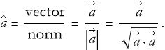
(16.143)

Say that we have two vectors, and that are perpendicular

If we add them we get the traditional sum of vectors

If we look at this long enough, it will occur to us that this forms a right triangle. We can treat the two vectors, and , as the base and altitude of the triangle and the hypotenuse is . If we apply the Pythagorean theorem, we can write,

(16.144)

We can rewrite this,

(16.145)

If the two vectors are not perpendicular then our diagram changes

Then (16.145) is no longer , but is some correction from ,

(16.146)

We can add a new vector to and we will call it ,

The new altitude vector will be renamed ,

We then rewrite (16.144)

(16.147)

If we use the Pythagorean theorem for the smaller triangle ,

(16.148)

We can now rewrite (16.146)

(16.149)

It turns out that the magnitude of a sum of vectors is

(16.150)

so (16.149) becomes

(16.151)

By using the definition of the scalar product we are left with

(16.152)

So what is this correction? It must depend on the angle between the vectors. When vectors are perpendicular this correction has a value of 0. Can we think of a value of an angle whose value is 0 when the angle is π/2 radians? One comes to mind, cos(π/2)=0.

The vector is called the projection of the vector onto the direction of the vector . How do we find θ? Starting from (16.141)

(16.153)

We can solve this,

(16.154)

If we have two column vectors, how do we find their scalar products. Say we have two arbitrary column vectors,

(16.155)

then the scalar product is

(16.156)

It turns out that the scalar product of parallel vectors is 1, and the scalar product of orthogonal vectors is 0.

So the scalar product becomes

(16.157)

For n-dimensional vectors we can generalize it,

(16.158)

It can get tiring to write the summation symbols all the time. We will adopt the Einstein summation convention, yes it is named after that Einstein, where any term that has the same superscript and subscript is assumed to be summed over all of the dimensions of the space. Thus,

(16.159)

To apply this to the scalar product we introduce a new symbol,

(16.160)

This is the Kronecker delta, named after Leopold Kronecker. In fact, one definition of the scalar product of two unit vectors is the Kronecker delta

(16.161)

We can now redefine the scalar product.

(16.162)

If we apply the Einstein summation convention, this becomes

(16.163)

There is a second product of vectors whose result is a vector, thus it is called the vector product. We will get to that a bit later. A third product of vectors results in a kind of matrix representation that is called a dyadic product, or a tensor product, we will get to this later.

Definitions

Definition 16.74 Scalar Product (Dot Product): The scalar product of two vectors and is a scalar given by where θ is the angle between the vectors.
Definition 16.75 Magnitude (Norm) of a Vector: The magnitude of a vector is

Definition 16.76 Unit Vector: A vector in the direction of   with magnitude 1,
Definition 16.77 Projection: The scalar projection of onto is .

Definition 16.78 Einstein Summation Convention: When an index appears once as a superscript and once as a subscript in a term, summation over that index is implied (repeated indices are summed).

Definition 16.79 Kronecker Delta: The symbol (or ) defined by .

Principles

Principle 16.31 Component Form of the Scalar Product: In components, the scalar product is

Principle 16.32 Perpendicular Vectors: Two vectors are perpendicular if and only if their scalar product is zero.

Theorems

Theorem 16.11 General Magnitude of Vector Sum: For any two vectors, .

Exercise 16.29: Prove Theorem 16.11

Theorem 16.12 Commutative Property of the Scalar Product:  

Proof of Theorem 16.12: This is a direct proof. By definition, the scalar product is where θ is the angle between the two vectors. Therefore, . Since the multiplication of real numbers is commutative, , it follows immediately that . QED

Exercise 16.30: Prove Theorem 16.12 using components.

Theorem 16.13 The Left-Distributive Property of the Scalar Product: .

Proof of Theorem 16.13: This is a direct proof. The scalar product equals the magnitude of times the projection of onto the direction of . That is,

(16.164)

Let . The projection of a sum of vectors onto a fixed direction is the sum of the individual projections (this follows from the linearity of projection, which is geometrically shown when you draw the vectors). Therefore,

(16.165)

Multiplying both sides by gives exactly . QED

Exercise 16.31: Prove Theorem 16.13 using components.

Theorem 16.14 Scalar Multiplication of the Scalar Product: .

Proof of Theorem 16.14: This is a direct proof. The scalar product . Multiplying by α stretches (or shrinks) its length by the factor ∣α∣ while keeping the direction the same (or reversing it if α<0). Therefore, the projection of onto the direction of is exactly α times the projection of onto the direction of . Hence, . QED

Exercise 16.32: Prove Theorem 16.14 using components.

Exercise 16.33: Begin with Definition 16.74 and copy it into your notebook. Reflect on its meaning for a few minutes. Note any thoughts that come to mind. How would you explain this to someone sitting in front of you. Write this down. Do this for each definition,  principle, theorem, and proof.

Exercise 16.34:
a) Let and be two vectors with magnitudes ∣ and ∣ and the angle between them is θ=60°.
    1) Compute the scalar product.
    2) What is the projection of onto ?
    3) If the vectors were perpendicular, what would the scalar product be?
b) Two vectors satisfy , , and .
    1) Use the general magnitude formula to find .
    2) Verify your answer using the law of cosines on the triangle formed by , , and .
    3)  What would be if the vectors are perpendicular?
c) The vector has components .
    1) Find and .
    2) Compute . What does this value represent physically?
    3) Find the projection of onto .
d) Let ,  and .
    a) Compute the scalar product.
    b) Rewrite the calculation using Einstein summation convention and the Kronecker delta.
    c) Verify that your result is the same.
e) Explain in your own words why the scalar product is called “scalar” while the vector product is called “vector.”

Vectors in Classical Mechanics

We have had many sections on classical mechanics spread through the various lessons. In classical mechanics we need to describe the location, motion, changes in the motion of objects, and the pushes or pulls that cause those changes. The most powerful and natural tool for doing all of this is a special kind of arrow that carries both magnitude and direction.

We begin with the question of where an object is. We choose a fixed reference point (usually the origin of our coordinate system) and draw an arrow from that point to the object’s location. This single arrow completely tells us the object’s position at any instant.

We call this arrow the position vector and denote it .

Next we ask how the object is moving. Take the small change in the position vector, . Divide this change by the corresponding time interval Δ t. The resulting arrow tells us the average rate and direction of motion during that interval. We call this the average velocity

(16.166)

When we make the time interval smaller and smaller, this average velocity arrow settles down to a definite arrow that describes the motion at that precise moment. We call this well-defined arrow the velocity vector .

If the velocity itself is changing, we repeat the process. The change in the velocity vector divided by a small time interval gives the average acceleration. When the time interval is made very small, we obtain the acceleration vector .

Now we come to the question of why the object accelerates. Something must be pushing or pulling on it. We represent every push or pull by an arrow whose length is proportional to the strength of the push or pull and whose direction shows the direction in which it acts. We call this arrow the force vector and denote it .

Definition 16.80 Position Vector: The arrow drawn from a chosen reference point to the location of an object at time t is called the position vector .

Definition 16.81 Velocity Vector: The velocity vector is the average velocity when the time interval gets small.

Definition 16.82 The Acceleration Vector: The acceleration vector is the average acceleration when the time interval  is taken to be very small.

Definition 16.83 Force Vector: The arrow that represents a push or pull, with length proportional to its strength and direction showing the direction in which it acts, is called the force vector .

One of the most important quantities in mechanics is the work done by a force. Work measures how much a force succeeds in moving an object in the direction of the force.

Take the force vector and the small displacement Δ that the object actually moves. The work done by the force during this small displacement is the scalar product of the two vectors

(16.167)

If the force is constant and the total displacement is Δ , then the total work is simply

(16.168)

This single expression automatically takes care of the angle between the force and the displacement so when they are in the same direction the work is maximum, when they are perpendicular the work is zero, and when they are opposite the work is negative.

We can write all of these vectors using components along the basis vectors

(16.169)

(16.170)

(16.171)

(16.172)

The work done then becomes

(16.173)

For example, a particle moves on a plane under a constant force that produces constant acceleration. Its position changes as

(16.174)

The velocity is constant at , and the acceleration is zero (no net force in this case, or maybe the forces balance).

Another example, a projectile is launched with initial velocity. A constant gravitational force produces acceleration . The velocity after time interval Δ t is

(16.175)

The position can be built by adding up the small changes .

The work done by gravity over any displacement is easily found using the scalar product with the gravitational force.

Exercise 16.35: Begin with Definition 16.80 and copy it into your notebook. Reflect on its meaning for a few minutes. Note any thoughts that come to mind. How would you explain this to someone sitting in front of you. Write this down. Do this for each definition.

Exercise 16.34:
a) A particle is located at coordinates (x, y, z) = (4, −3, 2) meters relative to the origin.
    1) Draw the position vector and write it in terms of the basis vectors.
    2) What is the magnitude of the position vector?
    3) Find the unit vector in the direction of .
b) During a time interval of 0.5 sec, a particle’s position vector changes from m to m.
    1) Compute the change in position.
    2) Find the average velocity vector.
    3) Find the average speed.
c) A particle moves so that its position at time t (in seconds) is meters.
    1) Find the change in position between 1 and 1.2 seconds.
    2) What is the average velocity over that time interval?
    3) If the velocity is changing, explain qualitatively what the acceleration vector must be doing.
d) A force of magnitude 20 N acts at an angle of 30° above the positive x-axis.
    1) Write the force vector in components.
    2) A displacement of m occurs while this force acts. Compute the work done using the scalar product.
    3) What would the work be if the force were perpendicular to the displacement?
e) Explain in your own words the difference between the position vector, velocity vector, and acceleration vector.

Ray Tracing in Optical Systems

Light carries information from one place to another. To understand how lenses, mirrors, and optical instruments work, we need a simple way to follow where a narrow beam of light goes. The best tool is to represent a narrow beam of light by a straight arrow. This arrow shows both the path the light takes and the direction in which it is traveling.

We call such an arrow a light ray (or simply a ray). The tail of the ray can be placed at any point along the path, and the direction of the arrow tells us the direction of travel. Because a ray has both magnitude (we can choose its length for convenience) and direction, it is a perfect example of a vector.

Definition 16.84 Light Ray: A straight arrow that represents the path and direction of travel of a narrow beam of light is called a light ray.

In ray tracing we follow one ray at a time through an optical system. At each surface (a mirror or the boundary between two materials) the ray may change direction. We use vectors to describe what happens.

When a ray strikes a smooth mirror, it bounces off. The law of reflection is very simple: the incoming ray, the outgoing ray, and the normal (a perpendicular arrow sticking straight out of the surface) all lie in the same plane, and the angle of incidence equals the angle of reflection.

Using vectors we can describe this neatly. Let be the unit vector in the direction of the incoming ray (pointing toward the mirror), and let be the unit normal vector pointing outward from the mirror surface. The reflected ray direction is given by reversing the component of the incoming ray that points along the normal

(16.176)

This single vector equation automatically gives the correct law of reflection.

When a ray crosses from one transparent material into another (for example, from air into glass), it bends. This bending is called refraction. The amount of bending depends on the two materials and the angle at which the ray hits the surface.

We again use the normal vector at the surface. The ray changes direction according to a simple geometric rule (Snell’s law), but the important point is that we can continue tracing the new ray direction after the bend using vector methods.

Definition 16.85 Ray Tracing: The technique of following the path of light rays through an optical system by applying the laws of reflection and refraction at each surface is called ray tracing.

Because rays are vectors, we can:

Add them or subtract them when combining paths,

Use the scalar product to find angles between rays and normals,

Keep track of position vectors to see exactly where each ray strikes the next surface.

This makes it straightforward to design and understand lenses, mirrors, telescopes, microscopes, and cameras.

For example, a ray strikes a flat mirror. Its incoming direction is . After reflection the new direction is (as wer have already stated)

The image appears behind the mirror exactly as far as the object is in front—a direct consequence of the vector reflection rule.

For another example, a ray parallel to the optical axis passes through a convex lens and is bent toward the focal point. Another ray passing through the center of the lens continues in a straight line. Where these two rays cross after the lens is the image point. We locate this point by tracing the rays as vectors.

Exercise 16.35:
a) A narrow beam of light travels from the point (0, 0) toward the point (3, 4).
    1) Draw the light ray as a vector and write it in component form.
    2) Find a unit vector in the direction of this ray.
b) A light ray with direction m strikes a horizontal mirror (whose outward normal is .
    1) Using the reflection formula , compute the direction of the reflected ray.
    2) Draw the incoming ray, normal, and reflected ray.
    3) Verify that the angle of incidence equals the angle of reflection.
c) An object is placed 5 cm in front of a plane mirror. A ray leaves the object at 30° to the normal.
    1) Draw the incident ray, reflected ray, and normal.
    2) Use vector ideas to explain why the image appears 5 cm behind the mirror.
    3) Where does the image appear to an observer looking into the mirror?
d) A light ray in air strikes a flat glass surface at an angle of 40° to the normal. The ray bends toward the normal inside the glass.
    1)  Draw the incident ray, refracted ray, and normal. Label the angles.
    2) Qualitatively explain why the ray bends toward the normal when entering glass from air.
    3) If the ray inside the glass makes an angle of 25° with the normal, what does this tell you about the relative speeds of light in air and glass?
e) Consider a thin convex lens with two important rays:
        A ray parallel to the optical axis,
        A ray passing through the center of the lens (undeviated).
    1) Draw both rays striking the lens and continuing after it.
    2) Where do these two rays cross after the lens? What does this point represent?
    3) Explain how ray tracing helps us locate the image without doing complicated calculations.
f) Why is it useful to treat light rays as vectors in optical systems?
g) A concave mirror forms a real image. Sketch the ray diagram using at least two rays and explain how the vectors help you locate the image.
h) Name two optical instruments (e.g., telescope, microscope, camera) that rely heavily on ray tracing and briefly explain the role of reflection or refraction in each.

Canonical Forms in Three Dimensions

In ray tracing we follow light rays through lenses, mirrors, and other optical components. Many of these components have curved surfaces—a lens might be part of an ellipsoid, a mirror might be part of a paraboloid, and some special surfaces (like hyperbolic mirrors) appear in advanced instruments. To understand and design such systems, we need a way to recognize the true geometric shape hidden inside a complicated equation.

The key insight is that any surface in three-dimensional space that can be described by a second-degree equation can be simplified by shifting and rotating the coordinate axes until the equation takes one of a small number of especially simple forms. Once the equation is in one of these simple forms, the shape of the surface becomes obvious at a glance.

We call these especially simple equations the canonical forms of quadric surfaces.

In three dimensions, a surface is described by a single equation relating x, y, and z. The most general second-degree equation in three variables is

(16.177)

By translating and rotating the coordinate axes, this equation can always be reduced to one of seventeen especially simple canonical forms we illustrate below.

1. Ellipsoid

(16.178)

This surface is a closed, bounded, oval-shaped figure—a stretched or squashed sphere. It looks like a football or a rugby ball.

2. Imaginary Ellipsoid

(16.179)

No real points satisfy this equation. It is called imaginary because it exists only in the complex domain. It serves as a useful mathematical placeholder when classifying surfaces.

3. Hyperboloid of One Sheet

(16.180)

This surface looks like a cooling tower or a hourglass that has been pinched in the middle but never quite closes. It is connected and extends to infinity in both directions along the z-axis. It has straight lines lying entirely on it, making it useful in engineering and optics.

4. Hyperboloid of Two Sheets

(16.181)

This surface consists of two separate bowl-shaped pieces facing away from each other. It is disconnected.

5. Second-Order Cone (real cone)

(16.182)

This is a double cone with its vertex at the origin. Conical mirrors and certain focusing devices make use of this geometry.

6. Imaginary Second-Order Cone

(16.183)

Only the origin satisfies this equation in real space. It is the imaginary counterpart of the real cone.

7. Elliptic Paraboloid

(16.184)

This surface looks like a bowl or a paraboloid dish opening upward. It is the classic shape of satellite dishes and reflecting telescope mirrors because parallel rays coming in reflect to a single focal point.

8. Hyperbolic Paraboloid

(16.185)

This surface has a saddle shape—it curves upward in one direction and downward in the other. It is a ruled surface with two families of straight lines on it. It appears in some advanced optical designs and in structural engineering (e.g., roofs).

9. Elliptic Cylinder

(16.186)

This surface is formed by taking an ellipse in the x y-plane and extending it straight up and down parallel to the z-axis. It looks like an infinite elliptical tube.

10. Imaginary Elliptic Cylinder

(16.187)

No real points satisfy this equation except in the complex sense. It is the imaginary version of the elliptic cylinder.

11. Pair of Intersecting Planes

(16.188)

This represents two planes that cross each other along a line (like the pages of an open book standing upright).

12. Pair of Intersecting Imaginary Planes

(16.189)

This has no real points except the z-axis and is considered imaginary.

13. Hyperbolic Cylinder

(16.190)

This surface looks like a pair of infinite curved walls facing away from each other, extending along the z-axis.

14. Parabolic Cylinder

(16.191)

This is a parabolic trough extending infinitely in the z-direction. It focuses light along a line rather than a point.

15. Pair of Parallel Planes

(16.192)

This represents two flat parallel planes (x = a and x = −a).

16. Pair of Imaginary Parallel Planes

(16.193)

These planes exist only in the complex domain.

17. Pair of Coincident Planes

(16.194)

This represents a single plane counted twice (x = 0 with multiplicity two).

Many of these surfaces—especially the hyperboloid of one sheet, the hyperbolic paraboloid, the cone, and all the cylinders—contain straight lines that lie entirely on the surface. These straight lines are called rectilinear generators. Their presence often simplifies manufacturing and optical design because light can travel along them or mechanical elements can be aligned with them.

Definition 16.86 Canonical Form: One of the seventeen especially simple second-degree equations obtained after translation and rotation of axes is called a canonical form of a quadric surface.

Definition 16.87 Rectilinear Generator: A straight line that lies entirely on a quadric surface is called a rectilinear generator.

By reducing any second-degree equation to one of these canonical forms, we immediately recognize the geometric nature of the surface. This recognition turns abstract algebra into concrete pictures we can use when designing optical systems, analyzing fields, or solving problems in theoretical physics.

Exercise 16.35:
a) Reduce each of the following equations to one of the seventeen canonical forms by completing the square or shifting coordinates, then name the surface:
    1)
    2)
    3)
    4)


b) Which of the following surfaces possess rectilinear generators (straight lines lying entirely on the surface)?
    1) Hyperboloid of one sheet
    2) Hyperbolic paraboloid
    3) Elliptic paraboloid
    4) Elliptic cylinder
c) Explain in your own words what it means when a canonical form is called “imaginary” (e.g., imaginary ellipsoid, imaginary elliptic cylinder). Why are these forms still important even though they have no real points?
d) Consider the general second-degree equation
    1) Reduce it to canonical form.
    2) Name the surface.
    3) Sketch a rough picture of what the surface looks like.
e) Why is it useful to reduce a complicated second-degree equation in three variables to one of the seventeen canonical forms?
f) Why is it useful to treat light rays as vectors in optical systems?
g) Give one example of a ruled surface (a surface with rectilinear generators) from the list of canonical forms and explain one practical advantage of having straight lines on a curved surface.

Matrix Approximations of Slope

We have already seen how to approximate the slope of a curve at a point by drawing a secant line between two nearby points and calculating the rise over the run. This gives us a good estimate of the true tangent slope when the two points are close together. Now we ask a deeper question: can we use the powerful language of matrices to organize and improve this kind of approximation? It turn out that the answer is yes. A matrix can compactly describe a linear change—exactly the kind of straight-line behavior we use when approximating a curve with a secant. By putting the changes in the coordinates into a simple rectangular array, we can handle the approximation in a clean, systematic way that extends naturally to two or three dimensions.

A small change in the input produces a small change in the output. We collect these changes into vectors and relate them using a matrix.

Definition 16.88 Matrix Approximation of Slope: A matrix that relates a small change in the input vector to the corresponding small change in the output vector is called a matrix approximation of slope (or a linear approximation matrix).

Suppose we have a function y=f(x) and we look at two nearby points, x and x+Δ x. The change in the output is Δ y=f(x+Δ x)−f(x). We can write this relationship in matrix form as

(16.195)

where m is the ordinary slope. This is a 1×1 matrix.

Consider a point (x,y) on a curve or surface. A small displacement produces a change in some quantity. We can organize the rates of change into a matrix. For a function of two variables, this matrix has two rows and two columns and is built from the divided differences in each direction.The beauty of this approach is that once we have the matrix, we can multiply it by any small displacement vector to get the approximate change in the output—instantly and for any direction.

Suppose we have a curve given by y=f(x). Near a point x=a, we compute

(16.196)

where m is the secant slope [f(x + Δ x)-f(x)]/Δ x. This is the simplest matrix approximation of slope.

When we allow motion in both x and y directions (for example, on a surface z=f(x,y), the matrix grows to 2 × 2 and contains the rates of change with respect to each variable. Multiplying this matrix by a small displacement vector (Δ x,Δ y) immediately gives the approximate change in z.

This matrix approach is a direct extension of the secant-line approximation we studied earlier. Instead of calculating one slope at a time, the matrix collects all the directional rates of change in one object. Using a matrix makes the approximation systematic, easy to compute, and ready to be combined with the vector methods we have already learned in classical mechanics and ray tracing.

Exercise 16.36:
a) Consider the function near the point x=2.
    1) Compute the ordinary slope (divided difference) using Δ x=0.1.
    2) Write this slope as a 1×1 matrix m.
    3) Use the matrix to approximate Δ x when Δ x=0.05. Compare with the true change.


b) A function of two variables is approximated near (2, 3) by the matrix .
    1) A small displacement is . Compute the approximate change in the output using matrix multiplication.
    2) What does each entry of the matrix represent?
    3) If you change only the x-coordinate by 0.1 (keeping y fixed), what is the approximate change?
c) Using the same matrix m from the previous exercise, compute the approximate change for three different small displacements:
    1)
    2)
    3)


d) The position of a particle is . A small change in position produces a change in potential energy approximated by the matrix . A displacement occurs.
    1) Compute the approximate change in potential energy.
    2) In which direction would a small displacement produce the largest increase in potential energy?
    3) What physical quantity does this matrix represent?
e) Explain in your own words why representing slope approximation with a matrix is more powerful than using a single number.
f) How does this idea connect the concepts of slope, vectors, and geometric transformations?
g) Give one example from optics or mechanics where a matrix approximation of slope would be useful.

Geometric Transformations in Matrix Language

In Lesson 12 we explored geometric transformations from a purely geometric point of view. We learned how to slide, stretch, rotate, and flip figures by thinking about what happens to each point. Now we add a powerful new tool—matrix language. The same transformations we drew by hand can be described compactly and computed efficiently using matrices.

The central idea remains the same, we take the position vector of a point and apply a consistent rule to obtain the new position vector. The difference is that the rule is now expressed as multiplication by a matrix. One matrix can transform an entire collection of points at once.

A matrix is a compact machine that takes a position vector as input and produces the transformed position vector as output.

Definition 16.89 Geometric Transformation in Matrix Language: A rule that transforms position vectors by matrix multiplication is called a geometric transformation in matrix language (or a linear transformation when it can be represented by matrix multiplication).

In Lesson 12 you learned to rotate a figure by a certain angle or scale it by a certain factor. Now we express those same operations as matrices.

To rotate every point counterclockwise by an angle θ, multiply the position vector by the rotation matrix

(16.197)

If you have a position vector , the rotated point is .

To stretch the figure by factor k in the x-direction and factor m in the y-direction, use the diagonal scaling matrix

(16.198)

Reflection across the x-axis is given by the simple matrix

(16.199)

One of the great advantages of the matrix approach is that successive transformations can be combined by matrix multiplication. If you first rotate by θ and then scale, the combined transformation is simply the product of the two matrices (in the reverse order of application). This is much cleaner than applying each geometric step separately.

In ray tracing we use these matrix transformations to rotate mirrors and lenses, change coordinate systems, or redirect bundles of rays. The geometric intuition you gained in Lesson 12 now has a powerful computational partner — matrix language.

Exercise 16.37:
a) The rotation matrix for 90° counterclockwise is .
    1) Apply R to the point (3, 1).
    2) Apply R to the point (1, 0). What does this tell you about the transformation?
    3) What single geometric operation does this matrix perform?


b) A function of two variables is approximated near (2, 3) by the matrix .
    1) A small displacement is .
    2) What does each entry of the matrix represent?
    3) If you change only the x-coordinate by 0.1 (keeping y fixed), what is the approximate change?
c) Using the same matrix m from the previous exercise, compute the approximate change for three different small displacements:
    1)
    2)
    3)


d) The position of a particle is . A small change in position produces a change in potential energy approximated by the matrix . A displacement occurs.
    1) Compute the approximate change in potential energy.
    2) In which direction would a small displacement produce the largest increase in potential energy?
    3) What physical quantity does this matrix represent?
e) Let R be the 90° rotation matrix from Exercise a and S the scaling matrix from Exercise b.
    1) Compute the combined matrix S ·R.
.    2) Apply the combined matrix to the point (1, 0).
    3) Describe the overall geometric effect of applying rotation first and then scaling.
f) A light ray is represented by the direction vector . It strikes a mirror that reflects across the line y = x.
    1)  Write the reflection matrix for this mirror.
    2) Compute the reflected direction vector.
    3) Explain how matrix transformations make ray tracing systematic.
g) Explain in your own words the advantage of describing geometric transformations with matrices rather than doing each point separately.
h) How does this matrix language connect to the geometric ideas you learned in Lesson 12?

Use WL to Visualize How Matrices Change the Coordinates of a Point in Space

We have learned that a matrix can describe a geometric transformation—rotation, scaling, reflection, and more. The matrix takes a position vector as input and produces a new position vector as output. Now we take the decisive step from abstract mathematics to concrete visualization. Wolfram Language (WL) lets us watch these transformations happen right in front of us.

The central idea is simple, pick a point, represent its position as a vector, multiply that vector by a transformation matrix, and see where the point moves. By repeating this process for many points, we can watch an entire figure change shape or orientation.

A matrix is a machine that transforms position vectors. Wolfram Language lets us feed points into that machine and immediately see the result. The command MatrixPlot[] lets us see the machine, while an ordinary plot lets us see what happens to the poi nt itself.

Before applying a matrix, it is often helpful to look at the matrix directly. The command MatrixPlot displays the matrix as a grid of colored squares, where the color and intensity show the size of each entry.

For example, the rotation matrix for 45° looks like this. Recall you can use [ESC]deg[ESC] to produce degrees.

The pattern of colors immediately tells you how the transformation stretches or rotates the coordinate directions.

Start with a point whose position vector is . Suppose we want to rotate it by 45° counterclockwise. The rotation matrix is

(16.200)

In Wolfram Language we can compute the new position and plot both points.

To see the full effect of a matrix, apply it to a whole collection of points. Here is a short program that shows a square being rotated and then scaled.

You can combine these tools: define a matrix, apply it to many points, plot the before-and-after figures, and use MatrixPlot to inspect the matrix itself. This workflow turns matrix transformations into something you can see and play with.

In applications the same approach lets you rotate optical elements, change coordinate systems, or follow how small displacements transform under a force law.

Exercise 16.37:
a) Define the point p = {3, 1}.
    1) Use RotationMatrix[90°] to rotate the point by 90° counterclockwise.
    2) Plot both the original and rotated points on the same graph using different colors.
    3) Use MatrixPlot on the rotation matrix. What pattern do you see?


b) Create the vertices of a unit square: original = {{0,0}, {1,0}, {1,1}, {0,1}, {0,0}}.
    1) Define a scaling matrix S = {{2, 0}, {0, 0.5}}.
    2) Apply S to every point in original using the /@ operator.
    3) Plot the original square in blue and the transformed figure in red on the same axes. Describe the change in shape.
c) Let R = RotationMatrix[45°] and S = {{1.5, 0}, {0, 0.8}}.
    1) Compute the combined matrix S . R.
    2) Apply the combined matrix to the square from b.
    3) Plot the original square, the rotated square, and the final transformed square. What is the overall effect?


d) Create three different 2×2 matrices: a rotation by 30°, a scaling matrix, and a reflection across the x-axis.
    1) Use MatrixPlot on each matrix with the option ColorFunction -> “TemperatureMap”.
    2) Write a short description of what each plot tells you about the transformation.
    3) Apply each matrix to the point {2, 1} and verify your visual intuition.
e) Let R be the 90° rotation matrix from Exercise a and S the scaling matrix from Exercise b.
    1) Compute the combined matrix S ·R.
.    2) Apply the combined matrix to the point (1, 0).
    3) Describe the overall geometric effect of applying rotation first and then scaling.
f) Take the letter “L” approximated by the points {{0,0}, {0,2}, {1,2}, {1,0.5}, {0,0.5}}.
    1) Choose any 2×2 matrix (for example a rotation by 60° or a shear matrix {{1, 0.5}, {0, 1}}).
    2) Apply the matrix to all points of the “L”.
    3)  Plot the original and transformed “L”. Write a one-sentence description of what happened.
g) Explain in your own words why MatrixPlot is useful when studying geometric transformations.
h) How does visualizing transformations with WL help connect the matrix language to the geometric ideas from Lesson 12?i)

Summary

Write a summery of this chapter.

For Further Study

Murray H. Protter, Charles B. Morrey, Jr., (1966), Analytic Geometry, Addison-Wesley Publishing Company, Second Edition (1975). This book covers a lot of the fine details we presented in this chapter.

A N Das, (2009), Analytic Geometry of Two and Three Dimensions, New Central Book Agency (P) Ltd, Revised Edition (2019). This is a very good presentation of a lot of the material we covered here, but in much greater detail.

Giovanni Landi, Alessandro Zampini, (2018), Linear Algebra and Analytic Geometry for Physical Sciences, Springer. The first four chapters cover the materials of this lesson.

William Wooton, Edwin F. Beckenbach, Frank J. Fleming, (1981), Modern Analytic Geometry. Houghton-Mifflin Company. This book is a good presentation, from an elementary point of view, of the material of this lesson.

Marshall C. Pease, III, (1965), Methods of Matrix Algebra. Academic Press. The first two chapters cover the material of this chapter.

Richard Bronson, (1989), Matrix Operations. McGraw-Hill Education, Schaum’s Outline Series. This is a very readable account and contains far more material than we covered here. It has a lot of problems solved in detail.

Alexander Altland, Jan von Delft, (2019), Mathematics for Physicists Introductory Concepts and Methods, Cambridge University Press. This is a fantastic book, the first three chapters cover the material of this chapter.

Analytical Geometry - The Basics (a compilation) by Maths with Mr. Thomas
https://www.youtube.com/watch?v=FWcenZstTjw
Excellent overview of distance, midpoint, gradient, and equations of lines — perfect starting point.

Vector Algebra playlist by MA Classes (Class 12 level, very clear)
Good for building intuition with examples.

Vectors | Chapter 1, Essence of Linear Algebra by 3Blue1Brown
https://www.youtube.com/watch?v=fNk_zzaMoSs
Beautiful geometric intuition (highly recommended for visual learners).

Introduction to Vector Spaces by Math with Richard (part of a full Linear Algebra course)
https://www.youtube.com/watch?v=DceiOHRrlN4
Clear and well-paced.

Linear Algebra - Matrix Operations by The Organic Chemistry Tutor or Postcard Professor
https://www.youtube.com/watch?v=p48uw2vFWQs
Quick, clear review of addition, multiplication, etc.

3Blue1Brown Essence of Linear Algebra series (especially chapters on matrix multiplication and linear transformations)
Best for intuition.