Lesson 14 Sets, Relations, and Functions
“The only way to learn mathematics is to do mathematics.” Paul R. Halmos
“Pure mathematics is, in its way, the poetry of logical ideas.” Albert Einstein
Introduction
We now enter the precise language that underlies all of modern physics and mathematics.
The collections of objects we study are sets, the ways objects are connected are relations, and the rules that assign one quantity to another are functions.
Everything we have done so far—points in space, physical quantities, units, scaling laws—can be described more powerfully and more generally with these three ideas.
A set is simply a collection of distinct objects. For example, the set of all points on a line, the set of all possible energies of a system, the set of all outcomes of an experiment.
A relation tells us how two objects are linked. For example, “Point A is to the left of point B,” “Particle X exerts a force on particle Y,” “Temperature ![]() is greater than temperature
is greater than temperature ![]() .”
.”
A function is a special relation that assigns exactly one output to each input. For example, distance as a function of time, force as a function of position, energy as a function of velocity.
These concepts are not abstract decorations—they are the working tools of mathematics and theoretical physics. The state space of a system is the set of all possible states it can be in. Forces are binary relations between objects (“A pushes B”).
We will prove classic results (De Morgan’s laws, properties of power sets, injectivity, surjectivity, bijectivity) not because they are “math for math’s sake,” but because they give us the logical precision to say exactly what we mean when we write a physical equation.
By the end of this lesson, you will see every physical law as a function, every conservation law as an equivalence relation, and every possible configuration of the universe as an element of a set.
Basic Concepts of Sets
If we take an abstract point of view, something important in theoretical physics, we can treat a unit of measurement as if it were an abstract box within which we could put anything at all for the purpose of counting similar objects. We can call such a box a cardinal number. This comes from the Latin, “cardinalis”, which means something pivotal or fundamental. Thus a cardinal number is the foundation of all of arithmetic. In this sense a cardinal number is a fundamental object of mathematics.
In general, in mathematics, we call a collection of mathematical objects a set. There is a vast literature about sets, and we will only use what we need of it. I recommend studying set theory beyond this lesson, as it is the basic language of modern mathematics. We have, in fact, just established a set, the set of all cardinals. We could also say that a cardinal number, say c, is a member or element of some set, say S. We would write this using the ∈ symbol for, “...is an element of the set...”, c∈S. We could also say that, “a is not an element of S,” a∉S. The number of elements that a set has is said to be the cardinal number of that set. A set having no elements is called the empty set or the null set; this is denoted Ø. A set having only one element is called a singleton set, you can represent it as the list of the single element, for example if the element is a we write {a}.
There are two ways to specify a set. The first way is to list all of its elements. For example, the set A is made up of the cardinal numbers 1, 2, and 3, we would write A={1,2,3}.
The second way of specifying a set is to write out the properties that are required for something to be considered a member of the set. We can symbolize such a property of an element of A by writing, p(a). Then we can construct the set by saying that A consists of all elements a such that p(a) is true. We can symbolize this using what is called set-builder notation.
![]()
(14.1)
Where the symbol of the vertical line represents the phrase, “...such that...”. We can have more than one property that defines the elements of a set. Say that we have both the property p(a) and the property q(a), then we can write the set
![]()
(14.2)
You can have as many properties as necessary. For example, we could say that we are considering all of the letters in the word "that":
![]()
(14.3)
here we are saying that there is some element that we label l that is an element of the word “that”. This does not mean that we are saying the letter l is part of the word “that”, it is only a label. This label can take on any of the elements of the set.
As another example, say that we have a set consisting of all counting numbers less than 5:
![]()
(14.4)
You will see that a lot mathematics involves developing new ways of writing things so they do not take up lots of space and time.
If you have two sets, A and B, and the set A is composed entirely of elements of the set B, then we say that set A is a subset of set B, we write this, A ⊆ B. Formally we write,
![]()
(14.5)
We can also say that B is the superset of A, and we can write B⊇A. If we can write A ⊆ B and B ⊆ A, then we say that the set A is equal to the set B, A=B. This means they have the same elements. If we impose the condition that a subset not be equal to the larger set, A≠B, then we say that the set A is a proper subset of the set B, A ⊂ B.
![]()
(14.6)
We can draw a picture where sets are represented by closed figures, and subsets are represented by intersecting closed figures. Such a representation is called a Venn Diagram.
Note that we are including intersection ∩ in this diagram, and we will not explain this until the next section.
There is a concept that we will discard in time. If we have a superset of all sets that we will consider, we can call that the Universe of Discourse, or just the universal set, we denote this as U.
Undefined Terms
Term 14.1 Set – A well-defined collection of distinct objects.
Term 14.2 Element / Member – An object that belongs to a set (∈).
Formal Definitions
Definition 14.1 Empty set / Null set – The unique set with no elements (Ø).
Definition 14.2 Singleton set – A set with exactly one element ({a}).
Definition 14.3 Set equality – Two sets are equal iff they have exactly the same elements. This is actually a statement of the Axiom of Extensionality.
Definition 14.4 Subset – A ⊆ B iff every element of A is in B (⊆). We can say that A is an inclusion of B.
Definition 14.5 Superset – A ⊇ B iff B contains every element of A (⊇).
Definition 14.6 Proper subset – A ⊂ B iff A ⊆ B and A ≠ B.
Definition 14.7 Venn diagram – Pictorial representation of sets and their relationships.
Definition 14.8 Universe of Discourse/Universal set – The superset of all sets you can consider.
Axioms
Axiom 14.1: The Axiom of Extensionality. Two sets are equal iff they have exactly the same elements. Formally, we write,
![]()
(14.7)
Principles
Principle 14.1: Any collection of distinct mathematical objects (numbers, points, physical quantities, cardinal numbers, etc.) can be regarded as a single unified entity called a set. Sets are the basic building blocks of modern mathematics and provide the language for all rigorous theoretical physics.
Principle 14.2: For any object x and any set S, exactly one of the following is true: x is a member (element) of S (written x ∈ S), or x is not a member of S (written x ∉ S). There is no third possibility—membership is definite and unambiguous.
Principle 14.3: The cardinal number of a set is the fundamental measure of its “size” by which we mean the number of distinct elements it contains. The empty set Ø has cardinal number 0 (the smallest cardinal), singleton sets have cardinal number 1, and so on. Cardinal numbers are themselves elements of sets and form the foundation of arithmetic.
Principle 14.4: A set can be defined in exactly two equivalent ways:
By explicit listing of its elements (called roster notation): A = {1, 2, 3}
By stating the defining property or properties that all elements must satisfy (called set-builder notation): A = {x | P(x)} or A = {x | P(x) ∧ Q(x)}.
These two descriptions always describe the same collection.
Principle 14.5 (Order and Repetition Do Not Matter) In a set, the order in which elements are listed is irrelevant, and no element is repeated. Thus {1, 2, 3}, {3, 1, 2}, and {1, 2, 2, 3} all represent exactly the same set.
Principle 14.6 (The Empty Set is Unique and Universal) There is exactly one empty set Ø — the set that contains no elements at all. It is a valid set in every context and serves as the starting point for constructing all other finite sets.
Principle 14.7 (Subset Relation is Hierarchical and Reflexive) If every element of set A is also an element of set B, then A is a subset of B (A ⊆ B). This includes the case A = B (every set is a subset of itself). If A ⊆ B and A ≠ B, then A is a proper subset of B (A ⊂ B). The subset relation organizes sets into a partial order.
Principle 14.8 (Equality of Sets is Determined by Elements Alone) Two sets A and B are equal (A = B) if and only if they have exactly the same elements — that is, A ⊆ B and B ⊆ A. No other property (order, labeling, or how the sets were constructed) matters.
Principle 14.9 (The Universe of Discourse is Context-Dependent) When working with sets in a particular problem, we often implicitly or explicitly restrict attention to a universal set U (the “universe of discourse”) that contains all elements we are willing to consider. All sets under discussion are understood to be subsets of this U. The choice of U is conventional and problem-specific.
Theorems
Theorem 14.1 The Empty Set is Unique
Proof of Theorem 14.1: Suppose there exist two empty sets, call them ![]() and
and ![]() . By definition, both have no elements. There is no x such that
. By definition, both have no elements. There is no x such that ![]() .There is also no x such that
.There is also no x such that ![]() . Now apply the Axiom of Extensionality so that for every x,
. Now apply the Axiom of Extensionality so that for every x,
![]()
(14.8)
in other words, both sides are false for any x. Therefore, by Extensionality, ![]() . Thus, any two empty sets must be equal, therefore the empty set is unique. QED.
. Thus, any two empty sets must be equal, therefore the empty set is unique. QED.
Theorem 14.2 The Empty Set is a Subset of All Sets
Proof of Theorem 14.2: Recall the definition of subset: A set A is a subset of B (written A ⊆ B) iff
![]()
(14.9)
Now let A = Ø. We must show,
![]()
(14.10)
The implication P ⇒ Q is true whenever P is false, recall this from the truth table of the implication. Here, the premise x ∈ Ø is always false (by the definition of the empty set). Therefore, the implication x ∈ Ø ⇒ x ∈ B is true for every x, regardless of B.Thus,
![]()
(14.11)
for any set B. QED.
Theorem 14.3 The Reflexivity of Subsets, A⊆A.
Proof of Theorem 14.3: Recall the definition of subset,
![]()
(14.12)
Now apply this to B = A. We need to show,
![]()
(14.13)
Let x be an arbitrary object. Consider the implication x ∈ A ⇒ x ∈ A. This statement is a tautology — it is always true, because the premise and conclusion are identical. If x ∈ A is true, then the conclusion x ∈ A is true. If x ∈ A is false, the implication is vacuously true (false premise). In either case, the implication holds. Since the implication is true for every x, the universal statement is true. Therefore A ⊆ A. QED
Theorem 14.4 The Transitivity of Subsets, If A⊆B∧B⊆C, then A⊆C.
Proof of Theorem 14.4: We use the definition of subset three times. By definition A⊆B means
![]()
(14.14)
and B⊆C means
![]()
(14.15)
We need to show that A⊆C,
![]()
(14.16)
Let x be an arbitrary object such that x ∈ A. From (14.14) we can say that x∈A⇒x∈B, so x∈B. From (14.15) we can say that x∈B⇒x∈C, so x ∈ C. Therefore x∈A→x∈C. Since this holds for every x, we have A⊆C. QED
Theorem 14.5 Antisymmetry of Subsets, If A⊆B and B⊆A, then A=B.
Sketch of the Proof of Theorem 14.5: By assumption: A⊆B ⇒ ∀x (x ∈ A ⇒ x ∈ B) and B⊆A ⇒ ∀x (x ∈ B ⇒ x ∈ A). Now take any x. If x ∈ A, ⇒ x ∈ B. If x ∈ B ⇒ x ∈ A. So x ∈ A ⇔ x ∈ B for every x. By the Axiom of Extensionality, A = B. QED
Exercise 14.1: Begin with Term 14.1 and copy it into your notebook. Reflect on its meaning for a few minutes. Note any thoughts that come to mind. How would you explain this to someone sitting in front of you. Write this down. Then do this for each term, definition, axiom, principle, theorem, and proof.
Exercise 14.2:
a) Give the details for the proof of the antisymmetry of sub sets.
b) Empty Set and Singleton Set:
1) Write the empty set in two different notations.
2) Write three different singleton sets that contain the number 5, a letter, and a point P.
3) Is {Ø} the same as Ø? Explain.
c) Subset vs Element: Let A = {1, 2, 3}. For each of the following, say whether it is an element of A or a subset of A (or both/neither):
2
{2}
Ø
{1, 3}
A itself.
d) Proper Subsets and Venn Diagrams: Let U = {1, 2, 3, 4, 5, 6, 7, 8} (the universal set). Let A = {1, 2, 3, 4}, B = {1, 3, 5}, C = {1, 3}.
1) List all proper subsets of C.
2) Draw a Venn diagram showing U, A, B, and C.
3) Which sets satisfy A ⊆ U, C ⊆ A, and C ⊂ B?
The Element-Chasing Method of Proof
This is the most common and most reliable way to prove almost anything about sets. To prove: Set A equals set B (or A ⊆ B, or any set equality/inclusion) you always do two things in this exact order:
Show A ⊆ B. Take an arbitrary element a that belongs to A.
Using the definitions and given facts, show that a must belong to B.
Show B ⊆ A. Take an arbitrary element b that belongs to B.
Using the definitions and given facts, show that b must belong to A.
When both directions are done, A = B (by extensionality).
If you only need A ⊆ B, you stop after step 2
For example, given ![]() and B={x∣∣x∣≤1} be subsets of the real numbers. We will use element-chasing to prove that B⊆A.
and B={x∣∣x∣≤1} be subsets of the real numbers. We will use element-chasing to prove that B⊆A.
Proof: Take an arbitrary element b∈B. By our definition of B, b∈B ⇒ {b}<=1.We can rewrite this -1<=b<=1. If we square these, we get, ![]() or
or ![]() . This also tells us that
. This also tells us that ![]() . By definition, this implies that b∈A. Since b is arbitrary, this implies that every element of B is also an element of A. Hence B⊆A. QED
. By definition, this implies that b∈A. Since b is arbitrary, this implies that every element of B is also an element of A. Hence B⊆A. QED
Exercise 14.3:
a) Let ![]() and B={x∈R∣∣x∣≤2}. Prove by element chasing that B⊆A.
and B={x∈R∣∣x∣≤2}. Prove by element chasing that B⊆A.
b) Let C={x∈Z∣x is divisible by 6} and D={x∈Z∣x is divisible by 2}. Prove by element chasing that C⊆D.
c) Let E={x∈R∣−3≤x≤5} and ![]() . Prove by element chasing that E⊆F.
. Prove by element chasing that E⊆F.
Set Operations
With the basic notion of sets now established, we introduce the ways to combine and compare them. These are the building blocks we will later use to describe the mathematical structures that make up all of theoretical physics.
If there is a set A, a rule, denoted *, that assigns to every pair of element a and b another element a*b is called a binary operation on A.
When we want to put together everything that belongs to either of two sets, we form their union. If we have sets A and B, their union is denoted with the symbol ∪, so we write A∪B. Formally we write,
![]()
(14.17)
We can visualize this with a Venn Diagram. Here we use the command to call a function from the online Function Repository, in this case we use VennDiagram.
![]()
When we want only what belongs to both sets at the same time, we form the intersection. We denote an intersection with the symbol ∩, so we write A∩B. Formally we write,
![]()
(14.18)
We can visualize it in a Venn diagram. Here we use the
Two sets whose intersection is the empty set are called disjoint.
The part of one set that is left after we remove everything that also belongs to another set is the difference. We denote the difference using the symbol -, so the difference of A from B is B - A. Formally, we write,
![]()
(14.19)
![]()
The elements that belong to exactly one of two sets (but not both) form the symmetric difference. We denote this with thew Δ symbol, se we write the difference of A from B, B Δ A, Formally we write
![]()
(14.20)
The Venn diagram looks like this.
![]()
When we have a fixed “everything” we are considering (thus we have established the universal set) and we want everything that is not in a given set, we take the complement. We denote this by an upper index c, for example, the complement of A is ![]() . Formally we write,
. Formally we write,
![]()
(14.21)
Changing the order of two sets does not change the result of union or intersection — we say they are commutative.
![]()
(14.22)
![]()
(14.23)
Grouping three sets in different ways does not matter for union or intersection—we say they are associative.
![]()
(14.24)
![]()
(14.25)
Union distributes over intersection and intersection distributes over union — this is distributivity.
![]()
(14.26)
![]()
(14.27)
Including the empty set changes nothing in union, and taking everything with the universal set changes nothing in intersection — these are the identity laws.
A set together with its complement gives everything, and a collection together with its complement gives nothing — these are the complement laws.
Doing the same operation twice on a set gives the same set—these are the idempotent laws.
The complement of a union is the intersection of the complements, and the complement of an intersection is the union of the complements—these are De Morgan’s laws.
When order matters in pairing elements from two sets, the corresponding elements form a set of ordered pairs.
The collection of all possible ordered pairs from two sets is the set called the Cartesian product. We write,
![]()
(14.28)
For example, a Venn diagram might show this situation,
where this would be written symbolically,
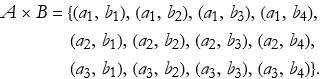
(14.29)
The Cartesian product of n sets is the set called the n-fold Cartesian product, its elements are called ordered n-tuples.
Definitions
Definition 14.9 Union: The collection of all elements that belong to at least one of two sets (A ∪ B).
Definition 14.10 Intersection: The collection of all elements that belong to both collections (A ∩ B).
Definition 14.11 Disjoint sets: Two collections with no elements in common (A ∩ B = Ø).
Definition 14.12 Set difference: Elements that belong to one collection but not another (A - B).
Definition 14.13 Symmetric difference: Elements that belong to exactly one of two collections (A △ B).
Definition 14.14 Complement: Everything (in the universal set) that is not in a given collection ![]() ).
).
Definition 14.15 Ordered pair: A pair where order matters ((a,b) ≠ (b,a)).
Definition 14.16 Cartesian product: All possible ordered pairs from two collections (A × B).
Definition 14.17 N-tuple: An ordered set containing n elements.
Definition 14.18 n-fold Cartesian product: All ordered n-tuples from n collections (A×B×...).
Theorems
Theorem 14.6 Commutativity of Union: A ∪ B=B∪A.
Proof of Theorem 14.6: We prove equality by showing both inclusions. First we need to show that A ∪ B ⊆ B ∪ A. Let a be an arbitrary element such that a ∈ A ∪ B. By the definition of a union, this means a ∈ A or a ∈ B. But this condition is the same as a ∈ B or a ∈ A. Therefore a ∈ B ∪ A. Since a was arbitrary, every element of A ∪ B is in B ∪ A. Thus A ∪ B ⊆ B ∪ A.
We now show that B ∪ A ⊆ A ∪ B. Let b be an arbitrary element such that b ∈ B ∪ A. Again, by the definition of union, b ∈ B or b ∈ A, which is the same as b ∈ A or b ∈ B. Therefore b ∈ A ∪ B. Since b was arbitrary, B ∪ A ⊆ A ∪ B.
Since both inclusions hold, we can use the Axiom of Extensionality to state A∪B=B∪A. QED
Theorem 14.7 Commutativity of Intersection: A ∩ B=B∩A.
Theorem 14.8 Associativity of Union: (A ∪( B∪C)=(A∪B)∪C.)
Proof of Theorem 14.8: We prove equality by element-chasing to show both inclusions. We begin with showing that (A ∪ B) ∪ C ⊆ A ∪ (B ∪ C). Let a be an arbitrary element such that
a ∈ (A ∪ B) ∪ C. By the definition of a union, this means a ∈ (A ∪ B) or a ∈ C.
We examine the first case where a ∈ (A ∪ B)⇒a∈A∨a∈B⇒a∈A ∪ (B ∪ C), since A is in the union, or B is inside B∪C.
For the second case, a ∈ C⇒ x ∈ A ∪ (B ∪ C) (because C is in the union)In both cases, a ∈ A ∪ (B ∪ C). Since a was arbitrary, (A ∪ B) ∪ C ⊆ A ∪ (B ∪ C).
Now we need to show A ∪ (B ∪ C) ⊆ (A ∪ B) ∪ C.
Let b be an arbitrary element such that b ∈ A ∪ (B ∪ C).
By the definition of union, b ∈ A or b ∈ (B ∪ C).
We examine the first case, b ∈ A⇒ b ∈ (A ∪ B) (because A is in A ∪ B). This implies b ∈ (A ∪ B) ∪ C.
We now turn to the second case, b ∈ (B ∪ C)⇒ b ∈ B or b ∈ C⇒ b ∈ (A ∪ B) (because B is in A ∪ B) or b ∈ C⇒ b ∈ (A ∪ B) ∪ C.
In both cases, b ∈ (A ∪ B) ∪ C.
Thus A ∪ (B ∪ C) ⊆ (A ∪ B) ∪ C.
Both inclusions hold, so by the Axiom of Extensionality A ∪ (B ∪ C) = (A ∪ B) ∪ C. QED
Theorem 14.9 Associativity of Intersection: (A ∩( B∩C)=(A∩B)∩C).
Theorem 14.10 Distributivity of Union over Intersection: (A ∪( B∩C)=(A∪B)∩(A∪C)).
Proof of Theorem 14.10: We shall prove equality by using element-chasing to show that both inclusions are true.
First we shall show A ∩ (B ∪ C) ⊆ (A ∩ B) ∪ (A ∩ C).
Let a be an arbitrary element such that a ∈ A ∩ (B ∪ C).By the definition of intersection, a ∈ A and a ∈ B ∪ C.
Since a ∈ B ∪ C, we have a ∈ B or a ∈ C.
For the first case, a ∈ B. Then a ∈ A and a ∈ B ⇒ a ∈ A ∩ B ⇒ a ∈ (A ∩ B) ∪ (A ∩ C).
We turn to the second case, x ∈ C. Then a ∈ A and a ∈ C ⇒ a ∈ A ∩ C ⇒ a ∈ (A ∩ B) ∪ (A ∩ C).
In both cases, a belongs to the right-hand side.
Now, since a was arbitrary, A ∩ (B ∪ C) ⊆ (A ∩ B) ∪ (A ∩ C).
We now show that (A ∩ B) ∪ (A ∩ C) ⊆ A ∩ (B ∪ C).
Let b be an arbitrary element such that b ∈ (A ∩ B) ∪ (A ∩ C).
Then b ∈ A ∩ B or b ∈ A ∩ C.
We now examine the first case, b ∈ A ∩ B⇒ b ∈ A ∧ b ∈ B⇒ b ∈ A ∧ (b ∈ B ∨ b ∈ C)⇒ b ∈ A ∩ (B ∪ C).
For the second case, b ∈ A ∩ C⇒ b ∈ A ∧ b ∈ C⇒ b ∈ A ∧ (b ∈ B ∨ b ∈ C)⇒ b ∈ A ∩ (B ∪ C).
In both cases, b ∈ A ∩ (B ∪ C).
Since b was arbitrary, (A ∩ B) ∪ (A ∩ C) ⊆ A ∩ (B ∪ C).
So both inclusions hold, thus by the Axiom of Extensionality A ∩ (B ∪ C)=(A ∩ B)∪(A ∩ C). QED
Theorem 14.11 Distributivity of Intersection over Union: (A ∩( B∪C)=(A∩B)∪(A∩C)).
Theorem 14.12 1st Complement law: ![]() .
.
Proof of Theorem 14.12: We show both directions using element-chasing.
For the first direction we show ![]() .
.
Take any element ![]() .
.
By the definition of union, a∈A or ![]() . If a∈A, then a∈U (because A⊆U).
. If a∈A, then a∈U (because A⊆U).
If ![]() , then
, then ![]() (because the complement is taken inside U).
(because the complement is taken inside U).
In either case, a∈U.
Therefore ![]() .
.
We now turn to the second direction where we need to show ![]() .
.
Take any element a∈U.
Either a∈A or a∉A.
If a∈A, then ![]() .
.
If a∉A, then by the definition of the complement ![]() , so again
, so again ![]() .
.
In both cases ![]() .
.
Therefore ![]() .
.
Both inclusions hold, so by the Axiom of Extensionality: ![]() . QED
. QED
Theorem 14.13 2nd Complement law: ![]() .
.
Theorem 14.14 De Morgan’s first law: ![]() .
.
Proof of Theorem 14.14: We prove the two sets are equal by showing each is a subset of the other.
First we show ![]() .
.
Let a be an arbitrary element such that ![]() .
.
By definition of the complement, x∉A ∪ B. This means it is not the case that a∈A or x∈B, so a∉A.Therefore (by the definition of complement) ![]() and
and ![]() , so
, so ![]() .
.
Since a was arbitrary, ![]() .
.
Secondly, we show ![]() .
.
We let a be an arbitrary element such that ![]() .
.
Then ![]() and
and ![]() , so a∉A and a∉B.
, so a∉A and a∉B.
Therefore a is not in A and not in B, so a∉A ∪ B.
By the definition of complement, ![]() .
.
Since a was arbitrary, ![]() .
.
Both inclusions hold, so by the Axiom of Extensionality ![]() . QED
. QED
Theorem 14.15 De Morgan’s second law: ![]() .
.
Theorem 14.16: A ∪ Ø = A.
Proof of Theorem 14.16: We show both directions by element-chasing.
For the first direction we show that A ∪ Ø⊆A. Let a be an arbitrary element such that a ∈ A ∪ Ø.
By the definition of union we have, a ∈ A or a ∈ Ø.
But nothing belongs to the empty set, so a ∈ Ø is impossible.
Therefore the only possibility is a ∈ A. Since a was arbitrary, every element of A ∪ Ø belongs to A.
Thus A ∪ Ø⊆A.
Next we show A⊆A ∪ Ø. Let a be an arbitrary element such that a ∈ A.
By the definition of union, every element that belongs to A automatically belongs to A ∪ Ø.
Therefore a ∈ A ∪ Ø.
Since a was arbitrary, every element of A belongs to A ∪ Ø.
Thus A⊆A ∪ Ø.
Both inclusions hold, so by the Axiom of Extensionality we have A ∪ Ø=A. QED
Theorem 14.17: A ∩ Ø = Ø.
Theorem 14.18: A ∪ U = U.
Proof of Theorem 14.18: Once again, we use the element-chasing method to show both inclusions.
We begin with the first inclusion, A ∪ U ⊆ U. Let a be an arbitrary element such that a ∈ A ∪ U.
By the definition of union, this means a ∈ A or a ∈ U.
If a ∈ A, then a ∈ U (because U contains every possible element).
If a ∈ U, then we are done with this argument.
In either case, a ∈ U.
Since a was arbitrary, every element of A ∪ U belongs to U, so A ∪ U ⊆ U.
We now turn to the second inclusion, U ⊆ A ∪ U. Let a be an arbitrary element such that a ∈ U.
Because U is the universal set, a certainly belongs to U.
Therefore a ∈ A ∪ U (the second part of the disjunction holds).
Since a was arbitrary, every element of U belongs to A ∪ U, so U ⊆ A ∪ U.
Since both inclusions hold, we conclude A ∪ U = U. QED
Theorem 14.19: A ∩ U = A.
Theorem 14.20: A × Ø = Ø × A = Ø.
Proof of Theorem 14.20: We use element-chasing to prove both directions for each equality.
We begin with A × Ø = Ø⇒ A × Ø ⊆ Ø.
Take any element (a, b) ∈ A × Ø.
By definition of Cartesian product, this requires b ∈ Ø.
But nothing belongs to the empty set, so there is no such b.
Therefore no ordered pair (a, b) can belong to A × Ø.
Hence A × Ø contains no elements at all, i.e. A × Ø = Ø.
We turn to this Ø ⊆ A × Ø.
The empty set is a subset of every set (there are no elements of Ø to violate the subset relation).
Thus Ø ⊆ A × Ø holds automatically.
Therefore A × Ø = Ø = Ø.
We now turn to this Ø × A = Ø.
Exactly the same argument, just swap the sets.
Take any supposed element (a, b) ∈ Ø × A.
Then a ∈ Ø and b ∈ A.
But a ∈ Ø is impossible so no such ordered pair exists. Therefore Ø × A = Ø.
Thus the Cartesian product with the empty set is always empty:A × Ø = Ø × A = Ø for any set A.
This is exactly analogous to how 0 is the absorbing (zero) element for multiplication, a · 0 = 0 · a = 0.
In set theory, Ø is the absorbing element for the Cartesian product. QED
Exercise 14.4: Begin with Definition 14.9 and copy it into your notebook. Reflect on its meaning for a few minutes. Note any thoughts that come to mind. How would you explain this to someone sitting in front of you. Write this down. Then do this for each definition, principle, theorem, and proof.
Exercise 14.5:
a) Give the details for the proof of Theorem 14.7. How does your proof compare to the listed proof of theorem 13.6?
b) Give the details for a proof of Theorem 14.9. How does your proof compare to the listed proof of theorem 13.8?
c) Give the details for a proof of Theorem 14.11. How does your proof compare to the listed proof of theorem 13.10?
d) Give the details for a proof of Theorem 14.13. How does your proof compare to the listed proof of theorem 13.12?
e) Give the details for a proof of Theorem 14.15. How does your proof compare to the listed proof of theorem 13.14?
f) Give the details for a proof of Theorem 14.17. How does your proof compare to the listed proof of theorem 13.16?
g) Give the details for a proof of Theorem 14.19. How does your proof compare to the listed proof of theorem 13.18?
h) Prove (A ∪ B) × C = (A × C) ∪ (B × C)
i) Prove (A ∩ B) × C = (A × C) ∩ (B × C)
j) Prove A × (B ∪ C) = (A × B) ∪ (A × C)
k) Prove A × (B ∩ C) = (A × B) ∩ (A × C)
l) Prove that if A × B = Ø, then either A = Ø or B = Ø (or both).
Geometric Sets
With set theory now giving us the precise language of modern mathematics, we return to geometry and discover that every geometric object is nothing more than a set of points. We begin with the plane (or three-dimensional space) itself. We treat the entire collection of all points we are considering as the universal set U. Every figure we draw is then a subset of this universal set of points. We can actually use another symbol for this set of all points, for the infinite line we call it the Euclidean space in one dimension, we symbolize this with the double-struck E, and we assign the number of dimensions as an upper index, ![]() . For the infinite place, we write
. For the infinite place, we write ![]() . For the infinite three-dimensional space (or simply three-space) we write
. For the infinite three-dimensional space (or simply three-space) we write ![]() .
.
A line segment joining two points A and B is the set of all points that lie between A and B, including A and B themselves. A ray starting at A consists of A together with every point extending infinitely in one direction from A. An entire straight line through A and B is the set of all points that lie on the infinite line passing through them. A circle with center O and radius r is the set of all points exactly distance r from O, while a filled disk includes every point at distance less than or equal to r. A triangle A B C is the set of all points inside and on the boundary of the three-sided figure formed by A, B, and C. A half-plane is the collection of all points lying on one side of a given line, either including the line or not, according to the definition we choose.
The familiar set operations now acquire vivid geometric meaning. The union of two regions contains every point that belongs to at least one of the regions; two overlapping disks, for example, form a union that includes both disks and their lens-shaped overlap. The intersection consists only of the points common to both regions; two intersecting lines yield one or two points, while two overlapping disks produce the lens itself. The set difference removes from one region everything that belongs to the other; subtracting a smaller disk from a larger one leaves a ring. The complement of a region, taken with respect to the whole plane or space, is simply the set of all points lying outside that region.
These operations obey the same algebraic laws we have already proved. Adding the empty set of points changes nothing, so a region united with the empty set remains itself. Intersecting any region with the empty set yields nothing. The union of a region with its complement fills the entire plane or space, while their intersection is empty. These identities are no longer abstract; they are visible facts about areas, volumes, and boundaries.
In physics, this viewpoint is extraordinarily powerful. The possible positions of a particle form a region of space representing a set of points. The trajectory of a moving particle is a curve itself another set of points. Two particles collide only if the sets representing their trajectories have a non-empty intersection. A physical state is an element of the vast set of all possible states. Forces, fields, and conservation laws all correspond to relationships among these geometric sets.
Geometry, seen through the lens of set theory, is no longer a collection of separate figures; it is a single, unified language in which every point, line, surface, and volume is a set, and every relationship among them is a set operation.
Definitions
Definition 14.19 Euclidean space (n-dimensional) ![]() : The universal set of all points in n-dimensional space subject to the rules of Euclidean geometry.
: The universal set of all points in n-dimensional space subject to the rules of Euclidean geometry.
Definition 14.20 Line segment joining points A and B: The set of all points lying on the line through A and B, including A and B.
Definition 14.21 Ray starting at A (in direction toward B): The union with all points extending infinitely in one direction from A along the line.
Definition 14.22 Straight line through A and B: The infinite set of all points collinear with A and B.
Definition 14.23 Circle with center O and radius r: The set of all points exactly distance r from O.
Definition 14.24 Filled disk (ball in 2D): The set of all points at distance ≤ r from O (circle plus interior).
Definition 14.25 Triangle ABC: The set of all points inside and on the boundary of the three-sided figure formed by segments AB, BC, CA (such figures can be called a convex hull including interior and boundary).
Definition 14.26 Half-plane: The collection of all points lying on one side of a given line (may or may not include the line, depending on closed/open choice).
Exercise 14.6: Begin with Definition 14.19 and copy it into your notebook. Reflect on its meaning for a few minutes. Note any thoughts that come to mind. How would you explain this to someone sitting in front of you. Write this down. Then do this for each definition.
Exercise 14.7:
a) Describe each of the following geometric sets using set notation and, when possible, draw a quick sketch.
All points in the plane that are exactly 5 units from the origin.
All points inside the square with vertices (0,0), (2,0), (2,2), (0,2).
All points on the line segment joining (−1, 3) and (4, −2).
The set of points (x, y) such that x ≥ 0 and y ≤ 1 (a closed half-plane corner).
b) Determine whether each set excludes its boundary (the set is open), includes its boundary (is closed). Justify your choice with a brief statement.
The disk of radius 2 centered at (0,0): ![]() .
.
The disk of radius 2 centered at the origin, ![]() .
.
c) Let ![]() , B = { (x,y) | |x| + |y| ≤ 1 }.
, B = { (x,y) | |x| + |y| ≤ 1 }.
Sketch both sets.
Describe A ∩ B geometrically (what shape is it?).
Describe A ∪ B geometrically.
d) Let I = [0, 1] and J = (2, 5).
Sketch I × J in the plane.
Is I × J open, closed, or neither?
What is the boundary of I × J?
Families of Sets
With the basic operations of union, intersection, and complement now mastered for two or three sets, we extend the idea to any number of sets—even infinitely many. A family of sets is simply a collection whose elements are themselves sets. We usually label the individual sets with an index that runs over some index set I. When I is finite, say {1, 2, …, n}, we write the family as ![]() . When I is infinite—for example, the natural numbers, the real numbers, or the set of all angles— we write {Aᵢ}ᵢ∈I or simply {Aᵢ}.
. When I is infinite—for example, the natural numbers, the real numbers, or the set of all angles— we write {Aᵢ}ᵢ∈I or simply {Aᵢ}.
The union of a family of sets is written
![]()
(14.30)
and contains every element that belongs to at least one of the sets in the family.
The intersection of a family is similarly written
![]()
(14.31)
and contains every element that belongs to all of the sets in the family simultaneously.
In words, the big ∪ is “or over all indices,” and the big ∩ is “and over all indices.”
Consider the family where ![]() , the set of the first n natural numbers. As n grows without bound, the union of all these sets is
, the set of the first n natural numbers. As n grows without bound, the union of all these sets is
![]()
(14.32)
the entire set of natural numbers, while their intersection is
![]()
(14.33)
because no single number belongs to every ![]() .
.
Now consider intervals centered at the origin. Let ![]() for every positive real number x. The union of all these open intervals is
for every positive real number x. The union of all these open intervals is
![]()
(14.34)
the entire real line, because any real number is inside some interval of large enough radius. Their intersection, however, is
![]()
(14.35)
because only the origin lies inside every interval, no matter how small x becomes.
Finally, imagine a rotating a half-plane around the origin. For every angle φ, let ![]() be the half-plane below the line at angle φ. The union of all these half-planes is
be the half-plane below the line at angle φ. The union of all these half-planes is
![]()
(14.36)
because every point lies below some rotated line. Their intersection is
![]()
(14.37)
because no point can lie below every possible line passing through the origin.
The beautiful duality of De Morgan’s laws extends unchanged to families:
![]()
(14.38)
and
![]()
(14.39)
Distributivity also survives, intersecting a fixed set A with an arbitrary union yields the union of the individual intersections, and uniting A with an arbitrary intersection yields the intersection of the individual unions,
![]()
(14.40)
and
![]()
(14.41)
In physics, families of sets appear everywhere. The collection of all possible positions of a particle at different times is a family indexed by time. The region reachable by a robot arm is the union of all positions its joints can attain. The region forbidden by multiple constraints is the intersection of the complements of the allowed regions. Indexed unions and intersections give us the language to speak precisely about all times, all energies, all directions, or all particles at once.
A family of sets is nothing more than a set whose elements happen to be sets — and with it, the algebra of sets becomes powerful enough to describe the entire universe of physical possibilities.
Terms
Term 14.3 Family of sets: A collection whose elements are themselves sets. Usually written as ![]() where I is an index set (can be finite, countable, or uncountable).
where I is an index set (can be finite, countable, or uncountable).
Definitions
Definition 14.27 Index set I: Any set used to label the individual sets in the family (e.g., I = {1,2,3}, N, ℤ, R, or the set of all angles).
Definition 14.28 Union of a family: ![]() (read: “the set of everything that is in some
(read: “the set of everything that is in some ![]() ”).
”).
Definition 14.29 Intersection of a family: ![]()
![]() (read: “the set of everything that is in all
(read: “the set of everything that is in all ![]() at once”).
at once”).
Definition 14.30 Empty family: A family with no sets at all. By convention: ∪ (empty) = Ø and ∩ (empty) = universe (the set we are working inside).
Definition 14.31 Partition of a set X: A family of non-empty sets ![]() } such that
} such that
(1) the ![]() are pairwise disjoint
are pairwise disjoint ![]() .
.
(2) their union is the whole set X: ![]() .
.
Theorems
Theorem 14.21 De Morgan’s Laws for arbitrary families:
![]()
![]() .
.
Proof of Theorem 14.21: Let ![]() be an arbitrary (possibly infinite or uncountable) indexed family of sets, all contained in some universal set X. De Morgan’s laws state
be an arbitrary (possibly infinite or uncountable) indexed family of sets, all contained in some universal set X. De Morgan’s laws state
![]()
(14.42)
and
![]()
(14.43)
where ![]() denotes the complement with respect to X.
denotes the complement with respect to X.
Proof of (14.42): ![]() . We prove set equality by showing mutual inclusion. We begin with the subset relation. Let
. We prove set equality by showing mutual inclusion. We begin with the subset relation. Let ![]() . By the definition of complement,
. By the definition of complement, ![]() . This means there is no index i∈I such that
. This means there is no index i∈I such that ![]() , i.e., for every i∈I, we have
, i.e., for every i∈I, we have ![]() . Thus
. Thus ![]() for every i∈I, so
for every i∈I, so ![]() .
.
We n ow turn to the superset relation. Let ![]() . Then
. Then ![]() for every i∈I, i.e.,
for every i∈I, i.e., ![]() for every i∈I. Therefore x belongs to none of the
for every i∈I. Therefore x belongs to none of the ![]() , so
, so ![]() . Hence
. Hence ![]() .
.
Since both inclusions hold, ![]() .
.
Proof of (14.43): ![]() . Again, we prove the mutual inclusion. We begin with the subset relation. Let
. Again, we prove the mutual inclusion. We begin with the subset relation. Let ![]() . Then
. Then ![]() .This means it is not true that x belongs to every
.This means it is not true that x belongs to every ![]() , i.e., there exists some i∈I such that
, i.e., there exists some i∈I such that ![]() . Thus
. Thus ![]() for that i, so
for that i, so ![]() .
.
We now turn to thew superset relation. Let ![]() . Then there exists some i∈I such that
. Then there exists some i∈I such that ![]() , i.e.,
, i.e., ![]() . So x fails to belong to at least one
. So x fails to belong to at least one ![]() , hence
, hence ![]() . Therefore
. Therefore ![]() .
.
So both inclusions hold, so ![]() .
.
The proofs rely only on the logical meanings of union (“there exists”) and intersection (“for all”), so they work for any index set I, finite or infinite.
These are sometimes called the generalized De Morgan’s laws; when I is finite (usually I={1,2} or {1,…,n}), they reduce to the familiar two-set or n-set versions taught in elementary set theory.
Thus, De Morgan’s laws are proven for arbitrary families of sets. QED
Theorem 14.22 Distributive laws (one set over arbitrary family)
![]()
![]() .
.
Proof of Theorem 14.22: Let ![]() } be an arbitrary indexed family of sets (where I can be any index set, possibly infinite), all are subsets of some universal set. Let B be any set. Our goal is to prove the two distributive laws. These hold even when I is infinite (the finite-case proofs are special cases).
} be an arbitrary indexed family of sets (where I can be any index set, possibly infinite), all are subsets of some universal set. Let B be any set. Our goal is to prove the two distributive laws. These hold even when I is infinite (the finite-case proofs are special cases).
Proof of Law 1: Intersection distributes over arbitrary unions. We seek to show both inclusions. We begin with the subset relation. Let ![]() . By the definition of intersection, x∈B and
. By the definition of intersection, x∈B and ![]() . The second condition means there exists some k∈I such that
. The second condition means there exists some k∈I such that ![]() . Thus x∈B and
. Thus x∈B and ![]() , so
, so ![]() . Therefore
. Therefore ![]() .
.
We now turn to the superset relation. Let ![]() . Then there exists some k∈I such that
. Then there exists some k∈I such that ![]() . So x∈B and
. So x∈B and ![]() , which implies
, which implies ![]() . Hence
. Hence ![]() .Thus, both inclusions hold, so equality holds.
.Thus, both inclusions hold, so equality holds.
I leave the proof Proof of Law 2 as an exercise.
Theorem 14.23 Monotonicity of union and intersection: If Aᵢ ⊆ Bᵢ for every i, then ![]() and
and ![]() .
.
Proof of Theorem 14.23: To prove ![]() , take an arbitrary element
, take an arbitrary element ![]() . By the definition of the arbitrary union, this means there exists some j∈I such that
. By the definition of the arbitrary union, this means there exists some j∈I such that ![]() . Since
. Since ![]() (by the given condition), it follows that
(by the given condition), it follows that ![]() . Therefore,
. Therefore, ![]() (by the definition of arbitrary union). Since x was arbitrary, this holds for all elements of
(by the definition of arbitrary union). Since x was arbitrary, this holds for all elements of ![]() , so
, so ![]() .
.
Exercise 14.8: Begin with Term 14.3 and copy it into your notebook. Reflect on its meaning for a few minutes. Note any thoughts that come to mind. How would you explain this to someone sitting in front of you. Write this down. Then do this for each term, definition, theorem, and proof.
Exercise 14.9:
a) Let ![]() , and in general
, and in general ![]() for every positive integer n. Write the union
for every positive integer n. Write the union ![]() and the intersection
and the intersection ![]() explicitly.
explicitly.
Write ![]() and
and ![]() explicitly. Is there any integer that belongs to infinitely many of the sets
explicitly. Is there any integer that belongs to infinitely many of the sets ![]() ?
?
b) Let ![]() be any family of sets (finite or infinite index set I). Prove the two infinite De Morgan laws (14.40) and (14.41) using element-chasing.
be any family of sets (finite or infinite index set I). Prove the two infinite De Morgan laws (14.40) and (14.41) using element-chasing.
c) A family of non-empty sets ![]() is a partition of a set X if they are pairwise disjoint:
is a partition of a set X if they are pairwise disjoint: ![]() where i ≠ j, and their union is the whole set:
where i ≠ j, and their union is the whole set: ![]() .
.
Decide which of the following families are partitions of ℝ (the real line). Check to see if these are partitions of R.
![]() for every integer n
for every integer n
![]() for every integer n
for every integer n
![]() for every integer n
for every integer n
d) Prove Theorem 14.22 Law 2.
e) Prove Theorem 14.23 for intersection.
Proof by Mathematical Induction
Many statements concern every positive integer. For example, “the sum of the first n natural numbers is n(n+1)/2,” “a set with n elements has ![]() subsets,” “a polygon with n sides has n−2 diagonals from one vertex,” and so on.
subsets,” “a polygon with n sides has n−2 diagonals from one vertex,” and so on.
Checking infinitely many cases one by one is impossible, so we need a single argument that covers all positive integers at once.
Say that you have arranged an infinite line of dominoes numbered 1, 2, 3, …. If domino 1 falls into its neighbor, and whenever domino k falls, it knocks over domino k+1, then every domino will fall, no matter how large its biggest number.
Mathematical induction is precisely this domino argument applied to the set of positive integers. We call this the Principle of Mathematical Induction. Let P(n) be a statement about the natural numbers n = 1, 2, 3, … There are two parts of this method. The first is called the base case, where we show that P(1) is true. The second part is called the inductive step where we prove that for every k ≥ 1, if P(k) is true, then P(k+1) is also true. If we can prove both of these, then P(n) is true for all natural numbers (or the whole numbers if you begin with 0).
The set of natural numbers N = {1, 2, 3, …} has two decisive properties guaranteed by the way the numbers are built. The first is that 1 belongs to N. Whenever a number k belongs to N, the next number k+1 also belongs to N.
So, suppose P(1) holds and the inductive step holds. Assume, for contradiction, that some natural numbers fail P. Let m be the smallest natural for which P(m) is false. By definition m cannot be 1 (this represents the base case). We can see that m cannot be larger than 1, because then m−1 is a smaller natural, P(m−1) is true (by choice of m), and the inductive step forces P(m) to be true—leading to a contradiction. Therefore no such m exists, and P(n) holds for all naturals n.
So, how do we actually write an inductive proof?
Prove the base case–Verify P(1) directly.
Prove the inductive step–Assume P(k) is true for some k ≥ 1 (this is called the induction hypothesis).
Using only that assumption, prove P(k+1).
Conclusion–By the principle of mathematical induction, P(n) is true for all naturals n.
For example, we can use this for the sum of the first n natural numbers. We begin by making the claim that
![]()
(14.44)
for every natural n. We perform step 1, establishing the base case, n = 1. This gives us
![]()
(14.45)
So, the base step is true.
We now try the inductive step. We begin this by assuming that (14.44) holds for n = k
![]()
(14.47)
Now we add k+1 to both sides:
(14.47)
If we realize that k+1=n, then this becomes (14.44), so we have proved it for all natural numbers. QED
Sometimes proving P(k+1) needs the statement to be true for all natural numbers from 1 up to k. We call this strong induction. We would write if P(1) is true and, whenever P(1), P(2), …, P(k) are all true, then P(k+1) is true and P(n) holds for every natural number n.
The domino picture still works; each new domino can be knocked over by one of the previous ones.
Undefined Terms
Term 14.4 Successor: The number following any number k, written k+1.
Definitions
Definition 14.32 Base case: The verification that the proposed theorem P is true for the value 1, often written P(1).
Definition 14.33 Inductive step (ordinary induction): Proof that for every k ≥ 1, if P(k) is true, then P(k+1) is true.
Definition 14.34 Induction hypothesis: The assumption that P(k) holds for some fixed k ≥ 1.
Definition 14.35 Strong induction: If P(1) is true and, whenever P(1), …, P(k) are all true, then P(k+1) is true, then P(n) is true for all n ∈ N.
Axioms
Axiom 14.2 Successor Axiom (Peano-style): Given 1 ∈ N, and if k ∈ N, then k+1 ∈ N.
Principles
Principle 14.10 Principle of Mathematical Induction: If P(1) holds and ∀k ≥ 1 [P(k) ⇒ P(k+1)], then P(n) holds ∀n ∈ N.
Principle 14.11 Well-Ordering Principle: Every non-empty subset of N has a least element.
Principle 14.12 Strong Induction Principle: If P(1) holds and ∀k ≥ 1 [ (P(1) ∧ … ∧ P(k)) ⇒ P(k+1) ], then P(n) holds ∀n ∈ N.
Theorems
Theorem 14.24 Standard Induction Theorem: If the base case P(1) is true and the inductive step holds, then P(n) is true for all natural numbers n.
Proof of Theorem 14.24: We will prove this using proof by contradiction. Assume the two hypotheses hold: P(1) is true, and ∀k≥1, P(k) ⇒ P(k+1).
Suppose, for the sake of contradiction, that the conclusion is false. That is, suppose there exists at least one natural number m such that P(m) is false. Let S={n∈N∣P(n) is false}. By our setup, S is non-empty. By the Well-Ordering Principle (every non-empty subset of the natural numbers has a least element), S has a smallest element. Call this smallest element m. So m is the smallest natural number for which P(m) is false.
Now consider two possibilities: Case 1: m=1. But this contradicts the base case, which states that P(1) is true. Since we are assuming that our hypothesis is false, this cannot be true. Therefore m≠1
Case 2: m≥2. Then m−1 is a natural number and m−1<m. Since m is the smallest element of S, m-1∉S. That is, P(m−1) is true. By the inductive step (with k=m−1), since P(m−1) is true, it follows that P(m) is true.
But this contradicts the fact that m∈S (i.e., P(m) is false).
In both cases we reach a contradiction. Therefore our initial supposition must be false: there is no natural number m for which P(m) is false.
Hence P(n) is true for every natural number n. QED
Theorem 14.25 Strong Induction: If the base case P(1) is true and the strong inductive step holds, then P(n) is true for all natural numbers n.
Proof of Theorem 14.25: We will prove this using proof by contradiction. Assume the two hypotheses hold: P(1) is true, and ∀k≥1, [P(1)∧P(2)∧···∧P(k)] ⇒ P(k+1).
Suppose, for the sake of contradiction, that the conclusion is false—that is, there exists at least one natural number m such that P(m) is false.
Let S={n∈N∣P(n) is false}.
By our supposition, S is non-empty. By the Well-Ordering Principle, S has a smallest element; call it m. So m is the smallest natural number for which P(m) is false. We now examine two cases:
Case 1: m=1. But the base case states that P(1) is true. Therefore 1∉S. This contradicts the assumption that m=1 is in S. Hence m≠1.
Case 2: m≥2. Then m−1 is a natural number and m−1<m. Since m is the smallest element of S, m−1∉S. That means P(m−1) is true. Moreover, because m−1≥1, all the statements P(1),P(2),…,P(m−1) are true (again, because any smaller number cannot be in S.
Now apply the strong inductive step with k=m−1: Since P(1)∧···∧P(m−1) holds, it follows that P(m) is true.
But this contradicts the fact that P(m) is false (i.e., m∈S).
In both cases we have reached a contradiction. Therefore the initial supposition is false: no such m exists. Hence P(n) is true for every natural number n. QED
Theorem 14.26 Inductive Equivalence Theorem: The Principle of Mathematical Induction, Strong Induction, and the Well-Ordering Principle are logically equivalent.
Proof of Theorem 14.26: We prove the equivalences by showing the cycle: Standard Induction ⇒ Strong Induction ⇒ Well-Ordering ⇒ Standard Induction. (This closes the loop; the other directions follow similarly.)
Part 1: Standard Induction ⇒ Strong Induction
Assume Standard Induction holds. Let Q(n) be the auxiliary statement: “P(m) is true for all m = 1, 2, …, n.”
Base case for Q: Q(1) says P(1) is true as given by the hypothesis for P.
Inductive step for Q: Assume Q(k) is true, i.e., P(1) through P(k) all hold.
By the strong inductive hypothesis for P (with this k), P(k+1) is true.
Therefore Q(k+1) holds (P(1) through P(k+1) are all true).
By Standard Induction applied to Q, Q(n) is true for all n.
Hence P(n) is true for all n.
Thus Standard Induction implies Strong Induction.
Part 2: Strong Induction ⇒ Well-Ordering Principle
Assume Strong Induction holds.
Let S be any non-empty subset of N. We must show S has a least element.
Define the statement R(n): “Every non-empty subset of N that contains a number ≤ n has a least element.”
Base case: R(1) is true because the only non-empty subset involving 1 is {1}, which has least element 1.
Strong inductive step: Assume R(1) through R(k) are all true (i.e., every non-empty subset bounded above by k has a least element).
Now consider any non-empty subset T of N that contains a number ≤ k+1.
If T has an element ≤ k, then by the induction hypothesis R(k), T has a least element.
If not, then the smallest possible element in T must be k+1 itself (since T is non-empty and has something ≤ k+1). Thus k+1 is the least element of T.
By Strong Induction, R(n) holds for all n.
In particular, taking n large enough to exceed any element of our original non-empty S, S has a least element.
Thus Strong Induction implies the Well-Ordering Principle.
Part 3: Well-Ordering Principle ⇒ Standard Induction
Assume the Well-Ordering Principle holds.
Let P(n) be any statement satisfying the hypotheses of Standard Induction: P(1) is true, and ∀k ≥ 1, P(k) ⇒ P(k+1).
Suppose, for contradiction, that P(n) is not true for all n. Let S={n∈N∣P(n) is false}.
Then S is non-empty. By Well-Ordering, S has a least element m.
If m = 1, this contradicts the base case P(1) being true.
If m ≥ 2, then m−1 < m and m−1 ∉ S, so P(m−1) is true. By the inductive step, P(m−1) ⇒ P(m), so P(m) is true. This contradicts m ∈ S.
Both cases yield a contradiction, so S must be empty. Therefore P(n) is true for all n ∈ N.
Thus Well-Ordering implies Standard Induction.
Since we have shown Standard ⇒ Strong ⇒ Well-Ordering ⇒ Standard, all three statements are logically equivalent.QED
Exercise 14.10: Begin with Term 14.4 and copy it into your notebook. Reflect on its meaning for a few minutes. Note any thoughts that come to mind. How would you explain this to someone sitting in front of you. Write this down. Then do this for each term, definition, axiom,principle, theorem, and proof.
Exercise 14.11:
a) Prove that ![]() for all n ≥ 1.
for all n ≥ 1.
b) Prove that ![]() for all positive integers n ≥ 10 (first check smaller n directly).
for all positive integers n ≥ 10 (first check smaller n directly).
c) Prove that any set with n elements has exactly ![]() subsets.
subsets.
d) Explain in your own words why the domino analogy captures induction perfectly.
Axioms of Set Theory
With set theory now serving as the foundation of all mathematics, we must ask: on what solid ground do we build this foundation?
At the end of the nineteenth century, naive set theory (sets defined by any property, as we have been dealing with them so far) led to paradoxes—the most famous being Russell’s paradox: “Is the set of all sets that do not contain themselves a member of itself?”
To eliminate these contradictions while preserving the power of set theory, Ernst Zermelo in 1908 proposed the first axiomatic system, later refined by Abraham Fraenkel and others. The resulting Zermelo–Fraenkel set theory with the Axiom of Choice—universally abbreviated ZFC—is today the standard foundation of mathematics.
All the set operations we have used so far can be proved from these axioms.
The ZFC Axioms are
Axiom 14.3 Axiom of Extensionality: Two sets are equal if and only if they have exactly the same elements.
Axiom 14.4 Axiom of the Empty Set: There exists a set with no elements (the empty set Ø).
Axiom 14.5 Axiom of Pairing: For any two objects a and b, there exists a set {a, b} that contains exactly a and b.
Axiom 14.6 Axiom of Union: For any set of sets F, there exists a set that contains exactly the elements of the sets in F ![]() ).
).
Axiom 14.7 Axiom of Power Set: For any set A, there exists a set whose elements are exactly all the subsets of A (the power set P(A)).
Axiom 14.8 Axiom of Infinity: There exists at least one infinite set (from which the natural numbers can be constructed).
Axiom 14.9 Axiom Schema of Separation (Comprehension): Given any set A and any definite property P(x), there exists a set containing exactly those elements of A that satisfy P(x).
Here we introduce an important definition.
Term/Definition 14.36 Function: Let A and B be sets. A function from A to B, written f: A → B, is a subset f of A × B such that for each a ∈A there exists at most one b ∈B such that (a, b)∈f. If (a, b)∈f, then we write b = f(a). We will see more about functions later in this lesson. Another word for a functions is a map.
Axiom 14.10 Axiom Schema of Replacement: If a definite function F maps elements of a set A to objects, then there exists a set containing exactly the images F(x) for x ∈ A.
Axiom 14.11 Axiom of Regularity (Foundation): Every non-empty set A has an element that is disjoint from A (this prevents sets from containing themselves).
Axiom 14.12 Axiom of Choice (AC): For any set of non-empty disjoint sets, there exists a set that contains exactly one element from each of them. This deceptively innocuous axiom has developed a great deal of controversy.
These axioms are very important. Extensionality gives us the definition of set equality we have used all along. Empty Set, Pairing, Union, Power Set allow us to construct all the sets we need in everyday mathematics. Infinity guarantees the existence of the natural numbers. Separation and Replacement let us define new sets from old ones safely. Regularity blocks the paradoxes that destroyed nave set theory. Choice is needed for many proofs.
ZFC is the quiet, invisible foundation on which the entire edifice of modern mathematics stands.
Theorems
Theorem 14.27 Extensionality Theorem: Two sets are equal if and only if they have exactly the same elements. This follows directly from the Axiom of Extensionality.
Proof of Theorem 14.27: In precise language Theorem 14.24 can we written that for any sets A and B, A=B ⇔ ∀x (x∈A⇔x∈B). This theorem is essentially a direct restatement of the Axiom 14.1 The Axioms of Extensionality, whose formal statement is, ∀(A∧B) ∧(∀x) (x∈A⇔x∈B) ⇒ A=B). We now seek to prove the “if and only if” theorem using the axiom. We prove the two directions separately. We begin with the direct implication, ⇒. If A=B, , then they have exactly the same elements. In virtually all modern set theories, the membership relation ∈ satisfies the substitution property (or “Leibniz’s law” for equality). Namely, : if two objects are equal, any property true of one is true of the other. In particular, for any object a ,if a∈A, then (by substitution) a∈B. If a∈B, then a∈A.
Thus a∈A⇔a∈B for every a, i.e., A and B have exactly the same elements. (This direction is sometimes called the “principle of substitutivity of equality” and is logically prior to, or built into, first-order logic with equality.)
We now turn to the other direction ⇐. If A and B have exactly the same elements, then A=B. We will now prove this. Assume (∀a) (a∈A⇔a∈B). This is precisely the hypothesis of the Axiom of Extensionality, whose conclusion is A=B.Therefore, by the Axiom of Extensionality, A=B.
We conclude that combining both directions, we have established the biconditional A=B ⇔ A and B have exactly the same elements.
This is why the Axiom of Extensionality is also called the principle that sets are determined by their elements—it tells us that the only thing that matters about a set is which objects belong to it. No additional structure, labeling, or history distinguishes two sets that contain exactly the same members. QED.
Theorem 14.28 Empty Set Theorem: There exists a unique set with no elements, denoted Ø.
Proof of Theorem 14.28: This proof will have two part, existence and uniqueness. We begin with the existence part. By Axiom 14.2 The Axiom of the Empty Set, there exists a set that contains no elements. We denote this set by Ø.(Some textbooks construct Ø instead of taking it as an axiom, for example by the axiom of infinity plus separation, or by taking a singleton of something and removing it—but the standard modern treatment simply postulates its existence.) We are done with part one.
We now turn to uniqueness. Suppose A and B are both empty sets. That means that ∀x (x ∉ A) ∧ ∀x (x ∉ B).We now use Axiom 14.1 The Axiom of Extensionality, where two sets are equal if and only if they have exactly the same elements. Since every element of A is an element of B (and this is trivially true, because there are no elements of A (a vacuous truth)). Every element of B is also an element of A—also vacuously true. Therefore, by the Axiom of Extensionality, A = B. Thus any two empty sets are the same set.
In conclusion, there exists exactly one set that has no elements, and we call it the empty set Ø. QED
Theorem 14.29 Singleton Theorem: For any object a, there exists a set {a} containing a as its only element.
Proof of Theorem 14.29: Once again we will prove this in two parts, existence and uniqueness. We begin with existence. By Axiom 14.3 The Axiom of Pairing, for any objects a and b, there exists a set whose elements are exactly a and b. That is, (∃S)( ∀y) (y ∈ S y = a ∨ y = b).To construct the singleton {x}, simply apply the axiom with a = b = x, so (∃S)( ∀y) (y ∈ S y = x ∨ y = x). This simplifies to (∃S)( ∀y) (y ∈ S y = x). Thus the set {x} exists. (Intuitively: every subset of A is obtained by “choosing” for each element of A whether it belongs or not. Replacement guarantees the result is a set.)More formally: consider the definable function on the set of all functions from A to {0,1} (the set of choice functions exists by other axioms). Map each such function f: A → {0,1} to the subset { a ∈ A | f(a) = 1 }. Replacement says the image of this function is a set, and that image is exactly the collection of all subsets of A. Call this set P(A). Then, by construction, X ∈ P(A) ⇔ X ⊆ A.
We now turn to uniqueness. Suppose A and B are both sets whose only element is x. That means (∀y) (y ∈ A y = x) and (∀y) (y ∈ B y = x). Now we apply Axiom 14.1 The Axiom of Extensionality. If something belongs to A, it must be x, and x certainly belongs to B. So, every element of B is an element of A. Symmetrically, the only thing in B is x, which is in A. Therefore A = B by Extensionality.
In conclusion there exists exactly one set that contains x and nothing else; we call it the singleton {x}. QED.
Theorem 14.30 Unordered Pair Theorem: For any objects a and b, there exists a set {a, b} containing exactly a and b as elements.
Proof of Theorem 14.30: This will again be a proof in two parts. We begin with the existence part. We build {x, y} using only the axioms we already have. By the Singleton Theorem, the sets {x} and {y} both exist. By the Axiom of Pairing, there exists a set that contains exactly the two objects {x} and {y} as elements. Call this set P such that P = {{x}, {y}}. If x = y, then P = {{x}}, which is fine. By the Axiom of Pairing again (applied to the objects x and y themselves), there exists a set that contains exactly x and y as elements.
However, most textbooks take a slightly longer but completely explicit route to avoid any doubt. Form the singleton {x} (and show it exists). Then form the singleton {y} (and show it exists). Form the ordered pair (x, y) in 1921 the famous Polish Mathematician Kazimierz Kuratowski’s produced a new definition of the ordered pair (x, y) ≔ {{x}, {x, y}}. The elements of this ordered pair are exactly {x} and {x, y}. Take the union of that ordered pair {x, y} =∪{{x}, {x, y}} = {x}∪ {x, y} = {x, y}. This union exists by the Axiom of Union. Thus {x, y} exists in all cases.
We now turn to the second part, uniqueness. Suppose A and B are both sets whose elements are exactly x and y. That means (∀z) (z ∈ A (z = x ∨ z = y))∧(∀z) (z∈B (z=x∨z=y)). By the Axiom of Extensionality, two sets are equal if and only if they have the same elements. Every element of A is an element of B (because the only possibilities are x and y, both of which are in B). So, every element of B is an element of A (by symmetry).
Therefore A = B.
In conclusion, for any x and y, there exists exactly one set that contains precisely x and y as its elements. We denote this unique set by {x, y}. QED
Theorem 14.31 Union Theorem: For any sets A ∧ B , the union A∪B exists as a set.
Proof of Theorem 14.31: We begin with the existence of the union. We are given a set C whose elements are themselves sets (i.e., C is a set of sets). We must construct the set that collects everything inside any member of C. Use the Axiom Schema of Replacement (or Separation, depending on the presentation). Consider the class expression {y | ∃A ∈ C (y ∈ A)}.By Replacement (applied to the definable rule that sends each A ∈ C to its elements), this class is itself a set. Call this set U. Then clearly x ∈ U ⇔ ∃A ∈ C (x ∈ A).Therefore the union exists. (Older textbooks use the Axiom of Union directly: there exists a set whose elements are all the elements of the elements of C. The modern treatment derives the same result from Replacement or Comprehension.)
We now turn to proving the uniqueness of the union. Suppose U and V are both unions of the same collection C. That is, x ∈ U ⇔ ∃A ∈ C (x ∈ A) and x ∈ V ⇔ ∃A ∈ C (x ∈ A).The right-hand sides are identical, so ∀x (x ∈ U ⇔ x ∈ V).By the Axiom of Extensionality, U = V.Therefore the union is unique. QED
Theorem 14.32 Power Set Theorem: For any set A, the power set 𝒫(A)—the set of all subsets of A—exists.
Proof of Theorem 14.32: We begin by proving existence. We need to show that the collection of all subsets of A actually forms a set. This will be a standard modern proof using the Axiom Schema of Replacement + Separation. Then, by the Axiom of Replacement (or Subsets Axiom Schema in some presentations), the class { x | x ⊆ A } is itself a set. Intuitively we realize that every subset of A is obtained by “deciding” for each element of A whether it belongs or not. Replacement guarantees the result is a set. More formally: consider the definable function on the set of all functions from A to {0,1} (the set of choice functions exists by other axioms). Map each such function f: A → {0,1} to the subset { a ∈ A | f(a) = 1 }. Replacement says the image of this function is a set, and that image is exactly the collection of all subsets of A. Call this set P(A). Then, by construction, X ∈ P(A) ⇔ X ⊆ A. Thus the power set exists.
We now turn to uniqueness. Suppose P and Q are both power sets of A. That is, X ∈ P ⇔ X ⊆ A and X ∈ Q ⇔ X ⊆ A. These are identical, so (∀X) (X ∈ P ⇔ X ∈ Q). By the Axiom of Extensionality, P = Q.Therefore the power set is unique. QED
Theorem 14.33 Subset Theorem / Separation Theorem: For any set A and any definite property φ(x), the subset { x ∈ A | φ(x) } exists as a set.
Proof of Theorem 14.33: We prove the existence and uniqueness of B using the Axiom Schema of Replacement, the Axiom of Union, and the Axiom of Extensionality.
We begin with existence. Start with the set A. Define a mapping that picks out the elements we want, for each x ∈ A, if f(x) holds, replace x with the singleton {x} (which exists by the Singleton Theorem), if f(x) does not hold, replace x with the empty set Ø (which exists by the Empty Set Theorem). By the Axiom Schema of Replacement, the collection of all these replacements forms a set, say C = { replacement of x | x ∈ A }. (Replacement guarantees that the image under this definable rule is a set.) Now apply the Axiom of Union to C, let B = ∪ C.By the definition of union, y ∈ B ⇔ there exists some singleton or Ø in C such that y belongs to it. The empty sets contribute nothing. The singletons {x} contribute exactly x, and only when f(x) held. Therefore B = { x ∈ A | φ(x) }.
We now turn to uniqueness, Suppose D is another set such that D = { x ∈ A | φ(x) }. Then ∀y (y ∈ B ⇔ φ(y) ∧ y ∈ A) ⇔ (y ∈ D). By the Axiom of Extensionality, B = D.
The Subset Theorem holds for any A and property f, the separated subset exists and is unique. QED
Theorem 14.34 Foundation / No Infinite Descent Theorem: There is no infinite descending ∈-chain … ![]() . No set is an element of itself (x ∉ x).
. No set is an element of itself (x ∉ x).
Proof of Theorem 14.34: Suppose, for contradiction, there is such an infinite descending chain, ![]() , (where ∋ means “contains as an element”). Let S be the set {
, (where ∋ means “contains as an element”). Let S be the set {![]() } (this exists by the Axiom of Infinity and Replacement, since we can enumerate the chain). S is nonempty (it has
} (this exists by the Axiom of Infinity and Replacement, since we can enumerate the chain). S is nonempty (it has ![]() , at least). By the Axiom of Foundation, there exists some y ∈ S such that y ∩ S = Ø.
, at least). By the Axiom of Foundation, there exists some y ∈ S such that y ∩ S = Ø.
That means no element of y belongs to S. But y must be one of the ![]() in the chain. Let’s say
in the chain. Let’s say ![]() . By the chain,
. By the chain, ![]() , and
, and ![]() (by the definition of S). So
(by the definition of S). So ![]() , which means y ∩ S ≠ Ø—this leads to a contradiction. Therefore no such infinite descending chain can exist.
, which means y ∩ S ≠ Ø—this leads to a contradiction. Therefore no such infinite descending chain can exist.
We no explore the converse, no infinite descent implies the axiom of foundation. Suppose every descending membership chain is finite (no infinite descent). Assume, for contradiction, there is a nonempty set A with no “foundational” element—every x ∈ A has some common member with A (x ∩ A ≠ Ø).Start with any ![]() (thus A is nonempty). Since
(thus A is nonempty). Since ![]() , pick
, pick ![]() .
.
Since ![]() , pick
, pick ![]() . And so on forever. This produces an infinite descending chain
. And so on forever. This produces an infinite descending chain ![]() —this leads to a contradiction that violates the no infinite descent assumption. Therefore every nonempty set must have a foundational element.
—this leads to a contradiction that violates the no infinite descent assumption. Therefore every nonempty set must have a foundational element.
We conclude that The Axiom of Foundation is exactly equivalent to the statement “there are no infinite descending membership chains.” With this axiom, the universe of sets is “well-founded”—every set has a clear hierarchy down to the empty set, with no bottomless pits. QED.
Theorem 14.35 Cartesian Product Theorem: For any two sets A and B, the Cartesian product A × B exists as a set.
Proof of Theorem 14.35: We prove existence and uniqueness separately. We begin with existence. We must build the set of all ordered pairs. We use the standard Kuratowski definition of ordered pair (x, y) ≔ {{x}, {x, y}}.This is a pure set built only from x and y using pairing and singleton, and it satisfies the crucial property {{x}, {x, y}} = {{u}, {u, v}} ⇔ x = u ∧ y = v. We now proceed in clean steps
For any fixed a ∈ A, the singleton {a} exists by the Singleton Theorem.
For any b ∈ B, the unordered pair {a, b} exists by the Unordered Pair Theorem.
Therefore the set {{a}, {a, b}} = (a, b) exists (again just pairing).
For fixed a ∈ A, consider the collection of all such pairs with first component a, { (a, b) | b ∈ B } = { {{a}, {a, b}} | b ∈ B }.This collection is a set by the Axiom Schema of Replacement applied to B (replace each b with the set {{a}, {a, b}}).Call this set a × B (this can be seen as a row of pairs corresponding to a). Now collect all the rows of pairs A × B ≔ ∪ { a × B | a ∈ A }.The set { a × B | a ∈ A } exists by Replacement applied to A. Its union exists by the Union Theorem. Therefore A × B exists as a set.
We now turn to uniqueness. Suppose C and D both satisfy (z ∈ C ⇔ z is an ordered pair (x, y) with x ∈ A, y ∈ B) and the same for D. Then C and D contain exactly the same elements, so C = D
by the Axiom of Extensionality.
So, for any sets A ∧ B, there exists exactly one set A × B = { (x, y) | x ∈ A, y ∈ B }. QED.
Exercise 14.12: Begin with Definition 14.36 and copy it into your notebook. Reflect on its meaning for a few minutes. Note any thoughts that come to mind. How would you explain this to someone sitting in front of you. Write this down. Then do this for each definition, axiom, theorem, and proof.
Exercise 14.13:
a) Prove that if two sets A and B have exactly the same elements, then A = B.
b) Using only the Axiom of Extensionality and the Axiom of Infinity (or Pairing + Separation), prove that there exists a set with no elements (i.e., ∃Ø).
c) Let A and B be arbitrary sets. Using the Pairing Axiom, prove that there exists a set whose elements are exactly A and B (i.e., {A, B} exists).
d) Let φ(x) be any formula with free variable x. Using the Axiom of Separation (Comprehension), prove that for any set A, the subset { x ∈ A | φ(x) } exists in ZFC.
e) Prove that for any set ![]() (a “family” or “set of sets”), the set
(a “family” or “set of sets”), the set ![]() exists using only the axioms already introduced (especially Union).
exists using only the axioms already introduced (especially Union).
State Space and Dynamics
The deepest idea in physics is this, “Every physical system, at any instant, is completely described by a single element in some huge set.” That set is called the state space (usually written Ω or S). Everything the system can ever be, every possible situation it can ever find itself in, is an element of Ω. Note that we are using the word space as an arena for the mathematical establishment of rules.
Two situations that differ in any physically measurable way are two different elements. Two situations that are absolutely indistinguishable are the same element.
The laws of physics are nothing more than rules telling you how that point moves inside the state space Ω as time passes.
But what is a state? A state is the list of everything you need to know about a system to study it in relation to the problem you are considering.
So, when studying the motion of a particle in three space we need to know its position in each of the three dimension, and also it corresponding velocities.
To know everything about a single particle, you need its exact position and its exact velocity at this instant. So the state space is the set of all possible (position, velocity) pairs
![]()
(14.48)
Note that this is a six-dimensional space.
For N particles you just take six coordinates per particle,
![]()
(14.49)
this turns out to be a huge-dimensioned Euclidean space, but not infinite.
So, did you get all of that? Let’s stake a step back. Imagine an abstract system that has only one state. We could think of it as a coin glued to the table—forever showing heads. Here the state-space consists of a single element—namely Heads (or just H)—because the system has only one state. Predicting the future of this system is extremely simple: Nothing ever happens and the outcome of any observation is always H.
The next simplest system has a state-space consisting of two points; in this case we have one abstract object and two possible states. Imagine a coin that can be either Heads or Tails (H or T).
In classical mechanics, we assume that systems evolve smoothly—without any jumps or interruptions. Such behavior is said to be continuous. Obviously you cannot move between Heads and Tails smoothly. Moving, in this case, necessarily occurs in discrete jumps. So let’s assume that time comes in discrete steps labeled by natural numbers. A world whose evolution is discrete could be called stroboscopic.
A system that changes with respect to some variable is called a dynamical system. All dynamical systems have a variable that the system changes with respect to, we can call this the evolutionary variable. Time is usually the evolutionary variable, but it need not be. A dynamical system consists of more than a space of states. It also entails a law of evolution, or we could call it a dynamical law. The dynamical law is a rule that tells us the next state given the current state.
One very simple dynamical law is that whatever the state at some instant, the next state is the same. In the case of our example, it has two possible histories: H H H H H H . . . and T T T T T T . . . . The first law specified that the arrow from H goes to H and the arrow from T goes to T. Once again it is easy to predict the future: If you start with H, the system stays H; if you start with T, the system stays T.
Another possible dynamical law dictates that whatever the current state, the next state is the opposite. You can still predict the future. For example, if you start with H the history will be H T H T H T H T H T . . . . If you start with T the history is T H T H T H T H . . . .
We can even write these dynamical laws in mathematical form. The number of variables describing a system are called its degrees of freedom. Our coin has one degree of freedom, which we can denote by the Greek letter sigma, σ. Sigma has only two possible values; σ=1 and σ=-1, respectively, for H and T. We also use a symbol to keep track of the time. When we are considering a continuous evolution in time, we can symbolize it with t. Here we have a discrete evolution and will use n. The state at time n is described by the symbol σ(n), which stands for σ at n.
Let’s write equations of evolution for the two laws. The first law says that no change takes place. In equation form we write,
![]()
(14.50)
In other words, whatever the value of σ at the nth step, it will have the same value at the next step.
The second equation of evolution has the form
![]()
(14.51)
implying that the state flips during each successive step.
In each case the future behavior is completely determined by the initial state, such laws are called deterministic. We can now assert, without proof, that all of the basic laws of classical physics are deterministic.
To make things more interesting, let’s generalize the system by increasing the number of states. Instead of a coin, we could use a six-sided die, where we have six possible states.
Now there are a great many possible laws, and they are not so easy to describe in words—or even in equations. One law says that given the numerical state of the die at time n, we increase the state one unit at the next instant n+1. That works fine until we get to 6, at which point the diagram tells you to go back to 1 and repeat the pattern. Such a pattern that is repeated endlessly is called a cycle. For example, if we start with 3 then the history is 3, 4, 5, 6, 1, 2, 3, 4, 5, 6, 1, 2, . . . . We’ll call this pattern Dynamical Law 1.
How do we write a mathematical expression for this?
![]()
(14.52)
seems like a good attempt. But wait a minute? What happens when n=6? We need to impose some rule that brings us back to 1, when n>6. We can wrap the right-hand side of the expression in a modulo operation, denoted ![]() .
.
![]()
(14.53)
The modulo operation tells us that once the evolution variable exceeds 6 it return back to 1. So the evolution is exactly what we want.
Dynamical Law 2 looks a little messier than the last case, but it’s logically identical—in each case the system endlessly cycles through the six possibilities. If we relabel the states, Dynamical Law 2 becomes identical to Dynamical Law 1.
Exercise 14.14: Relabel the diagram of Dynamical Law 2 so that it looks the same as Dynamical Law 1. To make this formally true write down the rules that transform the given states into the new states to make the diagram the same, what we call isomorphic. Such rules are examples of transformations.
Not all laws are logically the same. Consider Dynamical Law 3 where there are two cycles. If you start on one of them, you can’t get to the other. Nevertheless, this law is completely deterministic. Wherever you start, the future is determined. For example, if you start at 2, the history will be 2, 6, 1, 2, 6, 1, . . ., and you will never get to 5. If you start at 5 the history is 5, 3, 4, 5, 3, 4, . . ., and you will never get to 6.
Dynamical Law 4 has three cycles.
It would take a long time to write out all of the possible dynamical laws for a six-state system.
Terms
Undefined Terms
Term 14.5 System: The physical object or set of objects being studied.
Term 14.6 State of a System: A state is a complete description of a system at a given instant, containing all information necessary to predict the future evolution uniquely.
Term 14.7 Time: A variable representing the ordering of events in a system.
Definitions
Definition 14.37 State Space for Finite Systems: For a system with finitely many possible distinct situations, the state space Ω is a finite set whose elements are exactly the possible states.
Definition 14.38 Dynamical Law / Evolution Rule: A dynamical law is a function f : Ω → Ω that assigns to each current state σ(t) the unique next state σ(t+1) = f(σ(t)).
Definition 14.39 Deterministic System: A system is deterministic if its dynamical law is a well-defined function (exactly one next state for each current state, see the section on functions below).
Definition 14.40 Trajectory / Orbit: Given an initial state ![]() , the trajectory is the sequence
, the trajectory is the sequence ![]() also written σ(n+1) = f(σ(n)).
also written σ(n+1) = f(σ(n)).
Definition 14.41 Cycle: A sequence of distinct states ![]() is a cycle of length k. A fixed point σ = f(σ) is a cycle of length 1.
is a cycle of length k. A fixed point σ = f(σ) is a cycle of length 1.
Definition 14.42 Degrees of Freedom: The number of independent values needed to specify a state. For a finite-state system with C(Ω) = N, the number of degrees of freedom is N (where we are counting states).
Definition 14.43 Evolution Variable: A discrete time label n ∈ Z (or n ∈ N) that numbers the successive states.
Axioms
Axiom 14.13 Finite State Space: The system has only finitely many mutually distinguishable state variables.
Axiom 14.14 Determinism: There exists a definite rule that, given any state at step n, uniquely determines the state at step n+1.
Axiom 14.15 Time-Translation Invariance: The dynamical law does not change with time: f is the same function at every step.
Theorems
Theorem 14.36 Uniqueness of Trajectories: Let the dynamical law be a function f: S → S, where S is the state space (any set, finite or infinite, but we will only need that S is a set). Assume the system is deterministic in the strong sense, so for each current state x ∈ S there is exactly one next state f(x). Then, for any two trajectories that start from the same initial state remain identical forever. In other words, if σ and τ are two trajectories (sequences of states) satisfying ![]() and σ(n+1) = f(σ(n)), τ(n+1) = f(τ(n)) for all integers n ≥ 0, then σ(n) = τ(n) for every n ≥ 0.
and σ(n+1) = f(σ(n)), τ(n+1) = f(τ(n)) for all integers n ≥ 0, then σ(n) = τ(n) for every n ≥ 0.
Proof of Theorem 14.36: Here we perform a proof by mathematical induction (on the discrete time step n). We prove the statement P(n) implies σ(n) = τ(n) for all trajectories starting at the same ![]() . The base case (n = 0) is by assumption
. The base case (n = 0) is by assumption ![]() , so P(0) is true. We now turn to the inductive step where we assume P(k) is true for some fixed k ≥ 0. That is, σ(k) = τ(k). Apply the dynamical law f (this is a genuine function, so it gives the same output for the same input), σ(k+1) = f(σ(k)) = f(τ(k)) = τ(k+1). Thus P(k+1) is true. So, by mathematical induction, P(n) holds for all whole numbers n ≥ 0. Therefore σ(n) = τ(n) for every time step n. The trajectories are identical. QED.
, so P(0) is true. We now turn to the inductive step where we assume P(k) is true for some fixed k ≥ 0. That is, σ(k) = τ(k). Apply the dynamical law f (this is a genuine function, so it gives the same output for the same input), σ(k+1) = f(σ(k)) = f(τ(k)) = τ(k+1). Thus P(k+1) is true. So, by mathematical induction, P(n) holds for all whole numbers n ≥ 0. Therefore σ(n) = τ(n) for every time step n. The trajectories are identical. QED.
Theorem 14.37 Eventual Periodicity: Let S be a finite set and let f: S → S be any function (deterministic dynamical law on a finite state space).Then every trajectory is eventually periodic. In other words starting from any initial state ![]() , the sequence
, the sequence ![]() eventually repeats with some period p ≥ 1.
eventually repeats with some period p ≥ 1.
Proof of Theorem 14.37: We execute a mixed proof by contradiction and induction . We fix an arbitrary starting state ![]() . Consider the sequence defined by
. Consider the sequence defined by ![]() We will prove that this sequence must repeat some state. Assume, for the sake of contradiction, that all the terms are distinct
We will prove that this sequence must repeat some state. Assume, for the sake of contradiction, that all the terms are distinct ![]() are all different from one another. Define the sets
are all different from one another. Define the sets ![]() (the first n+1 states in the sequence). Because we assumed everything is distinct, C(Sₙ) = n + 1. Now consider the statement P(n)⇒C(Sₙ) = n + 1. We prove P(n) for all n by induction. We prove the base case (n = 0), where we have
(the first n+1 states in the sequence). Because we assumed everything is distinct, C(Sₙ) = n + 1. Now consider the statement P(n)⇒C(Sₙ) = n + 1. We prove P(n) for all n by induction. We prove the base case (n = 0), where we have ![]() , so
, so ![]() . So the base case is true. We now turn to the inductive step, assume P(k) holds, i.e. the first k+1 states are all distinct. The next state is
. So the base case is true. We now turn to the inductive step, assume P(k) holds, i.e. the first k+1 states are all distinct. The next state is![]() . By the contradiction assumption,
. By the contradiction assumption, ![]() is different from
is different from ![]() . Therefore
. Therefore ![]() has one more element than
has one more element than ![]() , so
, so ![]() . Thus P(k+1) holds.
. Thus P(k+1) holds.
By mathematical induction, P(n) is true for every whole number n. That means for every n we can find n+1 distinct states inside S. But S is a fixed finite set. Let N = C(S) be the total number of elements in S. Take n = N. Then P(N) says there are N+1 distinct states in the sequence, all belonging to S, so C(S) ≥ N+1. This contradicts the fact that S has only N elements. Therefore the assumption “all terms are distinct” is false. Hence there exist integers i < j such that ![]() . The sequence from position i onward then repeats forever with period p = j − i ≥ 1. The part before i (if any) is the transient. Thus the trajectory is eventually periodic. Since the starting state
. The sequence from position i onward then repeats forever with period p = j − i ≥ 1. The part before i (if any) is the transient. Thus the trajectory is eventually periodic. Since the starting state ![]() was arbitrary, this holds for every trajectory. QED.
was arbitrary, this holds for every trajectory. QED.
Theorem 14.38 Decomposition into Transient + Cycle: Let S be a finite set and f: S → S any function. Then, for every starting state ![]() , the trajectory
, the trajectory ![]() decomposes uniquely as transient (possibly empty) → cycle That is, there exist whole numbers t ≥ 0 (representing the length of the transient, possibly 0) and p ≥ 1 (representing the length of the cycle) such that:, the states
decomposes uniquely as transient (possibly empty) → cycle That is, there exist whole numbers t ≥ 0 (representing the length of the transient, possibly 0) and p ≥ 1 (representing the length of the cycle) such that:, the states ![]() are all distinct and none of them ever reappears later and
are all distinct and none of them ever reappears later and ![]() are also all distinct. Then
are also all distinct. Then ![]() . The sequence repeats the block of p states forever,
. The sequence repeats the block of p states forever, ![]() for all k ≥ 0. Moreover, this decomposition is unique: t and p are completely determined by the trajectory.
for all k ≥ 0. Moreover, this decomposition is unique: t and p are completely determined by the trajectory.
Proof of Theorem 14.38: Our proof uses only the previous eventual periodicity result and finiteness. We already proved that every trajectory is eventually periodic. So there exist whole numbers m ≥ 0 and p ≥ 1 such that ![]() and the sequence repeats every p steps from position m onward. Now, lLet
and the sequence repeats every p steps from position m onward. Now, lLet ![]() . From step m onward the trajectory is
. From step m onward the trajectory is ![]() Because the whole trajectory is eventually periodic with period p starting at m, the cycle is exactly the set
Because the whole trajectory is eventually periodic with period p starting at m, the cycle is exactly the set ![]() . All p states in C are distinct (otherwise the period would be smaller). Now define the transient length t as the smallest whole number such that
. All p states in C are distinct (otherwise the period would be smaller). Now define the transient length t as the smallest whole number such that ![]() . Such a t exists because the trajectory eventually enters the repeating part (at latest at step m). We claim that the states
. Such a t exists because the trajectory eventually enters the repeating part (at latest at step m). We claim that the states ![]() are all distinct and none belongs to C. Then
are all distinct and none belongs to C. Then ![]() is the first state that lies on the cycle C.
is the first state that lies on the cycle C.
We now prove that claim, suppose two states in the transient were equal, say ![]() with 0 ≤ i < j < t. Then the trajectory would already be periodic with period j−i before reaching the cycle—but then the eventual period would start earlier, contradicting the definition of t as the first hitting time of C. Now suppose some
with 0 ≤ i < j < t. Then the trajectory would already be periodic with period j−i before reaching the cycle—but then the eventual period would start earlier, contradicting the definition of t as the first hitting time of C. Now suppose some ![]() belonged to C. Then the trajectory would have entered C at step k < t, again contradicting the minimality of t. Therefore the transient really is a chain of distinct states leading into the cycle, and it never loops back or re-enters the cycle early. Finally, the uniqueness of t and p where t is uniquely determined as the first time the trajectory hits the eventual cycle. So, p is uniquely determined as the minimal positive period of the tail (or equivalently the number of distinct states in the cycle).
belonged to C. Then the trajectory would have entered C at step k < t, again contradicting the minimality of t. Therefore the transient really is a chain of distinct states leading into the cycle, and it never loops back or re-enters the cycle early. Finally, the uniqueness of t and p where t is uniquely determined as the first time the trajectory hits the eventual cycle. So, p is uniquely determined as the minimal positive period of the tail (or equivalently the number of distinct states in the cycle).
Corollary 14.1: Let S be a finite set and f: S → S any function. Then the entire dynamics decomposes to the state space S is the disjoint union of
One or more cycles
Transient chains (possibly of length 0) that feed into those cycles.
From every state x ∈ S, after finitely many steps you reach a cycle, and once on a cycle you stay there forever.
In short every trajectory consists of a transient followed by a cycle, and there are no other possibilities.
Proof of Corollary 14.1: Take any state x ∈ S (it does not matter which one). Consider its trajectory ![]() By the Eventual Periodicity Theorem this trajectory is eventually periodic. That is, there exist t ≥ 0 and p ≥ 1 such that
By the Eventual Periodicity Theorem this trajectory is eventually periodic. That is, there exist t ≥ 0 and p ≥ 1 such that ![]() . Let
. Let ![]() . Then from y onward the trajectory is purely periodic with period p,
. Then from y onward the trajectory is purely periodic with period p, ![]() So y lies on a cycle of length p. Therefore, starting from x, after exactly t steps we reach the cycle, and we stay on it forever. Since x was arbitrary, this holds for every state in S. The transient part (the first t states, if t > 0) never returns, and the cycle part repeats forever. Moreover, different cycles are disjoint (because if two cycles shared a state, the trajectories would merge and become the same cycle). Thus the whole finite set S breaks cleanly into disjoint cycles, plus transient states that flow irreversibly into one of the cycles.
So y lies on a cycle of length p. Therefore, starting from x, after exactly t steps we reach the cycle, and we stay on it forever. Since x was arbitrary, this holds for every state in S. The transient part (the first t states, if t > 0) never returns, and the cycle part repeats forever. Moreover, different cycles are disjoint (because if two cycles shared a state, the trajectories would merge and become the same cycle). Thus the whole finite set S breaks cleanly into disjoint cycles, plus transient states that flow irreversibly into one of the cycles.
There are no exceptions, no wandering states, no chaos — everything eventually settles into perfect repetition. QED.
Theorem 14.39 Existence of Fixed Points or Cycles: Let S be a finite non-empty set and f: S → S any function. Then the dynamics necessarily contains at least one cycle (and this may have length 1, i.e., a fixed point, or length p ≥ 2). In particular, there exists at least one state x ∈ S such that ![]() for some whole number p ≥ 1. In everyday language we write every finite deterministic system has at least one periodic orbit (either a state that stays forever the same, or a loop that repeats forever).
for some whole number p ≥ 1. In everyday language we write every finite deterministic system has at least one periodic orbit (either a state that stays forever the same, or a loop that repeats forever).
Proof of Theorem 14.39: We already proved that every trajectory is eventually periodic. Now pick any state—for example, pick an arbitrary state z ∈ S (S is non-empty, so this is possible). Follow its trajectory, ![]() By the earlier theorem, this trajectory eventually enters a cycle. That cycle is a periodic orbit contained in S. Therefore at least one cycle exists. QED.
By the earlier theorem, this trajectory eventually enters a cycle. That cycle is a periodic orbit contained in S. Therefore at least one cycle exists. QED.
Exercise 14.15: Begin with Term 14.5 and copy it into your notebook. Reflect on its meaning for a few minutes. Note any thoughts that come to mind. How would you explain this to someone sitting in front of you. Write this down. Then do this for each term, definition, axiom, theorem, and proof.
Exercise 14.16:
a) A toy robot can be either Awake (A) or Asleep (S). Every minute it follows this rule: If it is Awake, it falls Asleep in the next minute. If it is Asleep, it wakes up (becomes Awake) in the next minute.
Draw the state-transition diagram (two circles, arrows).
Write the dynamical law in words and in mathematical form using σ(n) = A or S.
Starting from Awake, write the history for the first 6 steps.
Write the law using numbers (let A = 0, S = 1) and the modulo operation so it works for any n.
b) A traffic light for pedestrians cycles through four colors in this exact order and then repeats:Green → Yellow → Red → Blinking-Red → Green → …Label the states 1 = Green, 2 = Yellow, 3 = Red, 4 = Blinking Red
Draw the state-transition diagram.
Write the dynamical law using the style of Dynamical Law 1 in your notes (σ(n+1) = σ(n) + 1 with wrap-around).
Starting from Red (state 3), what state is it after 23 minutes?
Write the same law using the modulo operator (you may use mod 4, remembering that many languages count 0–3 instead of 1–4—both are acceptable if you are consistent).
c) Relabel the diagram of Dynamical Law 2 so that it looks the same as Dynamical Law 1. To make this formally true write down the rules that transform the given states into the new states to make the diagram the same, what we call isomorphic. Such rules are examples of transformations.
d) Can you think of a general way to classify the laws that are possible for a six-state system?
e) A beetle walks on the vertices of a regular hexagon labeled 1,2,3,4,5,6 clockwise.
At every step it always moves two vertices clockwise.Examples: 1 → 3, 3 → 5, 5 → 1, 2 → 4, etc.Draw the diagram. You will discover there are actually three separate cycles. What are they? Write the dynamical law with the simplest arithmetic expression + modulo that works for all starting positions. Starting from position 6, write the sequence until it loops. How many steps until it returns to 6? Is this system ergodic (can you reach any state from any other state)? Explain in one sentence.
f) Consider again six states arranged in a circle: 1-2-3-4-5-6. This time the rule is: From an odd-numbered state go to the next even (1→2, 3→4, 5→6) From an even-numbered state go to the next odd two steps ahead (2→5, 4→1, 6→3)
Draw the complete transition diagram (you should obtain exactly two disjoint cycles of length 3).
Try to write a single formula of the type σ(n+1) = something with modulo that works for all six states (most people find it impossible with one formula).
Now write two separate formulas: one that applies when σ(n) is odd, one when it is even (this is allowed and is exactly what the book does in more complex cases).
Choose a starting state (e.g., 1) and list the history. After how many steps are you guaranteed to return to the starting state no matter where you began?
Power Sets
With the idea of a set now firmly established, we meet one of the most astonishing constructions in all of mathematics: the power set. As we saw in ZFC axioms the power set of a set A, written P(A) or ![]() , is the set whose elements are all possible subsets of A—including the empty set and A itself.
, is the set whose elements are all possible subsets of A—including the empty set and A itself.
If A has n elements, then P(A) has exactly ![]() elements. This explosive growth—from n objects to
elements. This explosive growth—from n objects to ![]() subsets—is why the power set is often denoted
subsets—is why the power set is often denoted ![]() where each element of A can either be “in” or “out” of a subset, giving two choices per element.
where each element of A can either be “in” or “out” of a subset, giving two choices per element.
For example, If A = Ø, then P(Ø) = { Ø } has one element. To be clear, the cardinal number of Ø is 0, but its power set has cardinal number 1. If A = {a}, then P(A) = { Ø, {a} } has two elements. If A = {a, b}, then P(A) = { Ø, {a}, {b}, {a,b} } has four elements. If A = {1, 2, 3}, then P(A) has ![]() elements.
elements.
The pattern is unbreakable ![]() for any finite set A.
for any finite set A.
Every property, every condition, every question we can ask about elements of A corresponds to a subset of A. “All even numbers” → subset of integers, “All points inside the circle” → subset of the plane, “All allowed energies” → subset of possible energy values.
The power set is therefore the set of all possible properties that elements of A can satisfy.
Think of the plane as the universal set U. The power set P(U) contains every possible region you could ever draw—every point, every line segment, every triangle, every disk, every imaginable shape—because every shape is just a subset of points.
The power set shows that “all possible collections” is vastly larger than the original set. Even a tiny set of 10 elements has a power set with 1024 members; a set of 100 elements has a power set larger than the number of atoms in the observable universe.
In physics, the power set of the state space contains every conceivable physical situation—the ultimate catalogue of everything that could ever happen.
The power set is the mathematical embodiment of the idea that from simplicity explodes into a vast number of outcomes.
Definitions
Definition 14.44 Power Set of the Set A (![]() : The set whose elements are all possible subsets of A. That is, P(A)={B∣B⊆A}.
: The set whose elements are all possible subsets of A. That is, P(A)={B∣B⊆A}.
Theorems
Theorem 14.40: Ø ∈ P(A) and A ∈ P(A) for any A.
Proof of Theorem 14.40: We know that the empty set is always a subset of any set. Naively, A is always a subset of itself. To show that A ⊆ A, we must verify that every element of A is an element of A. This is obviously true (if x ∈ A, then x ∈ A). Therefore A ⊆ A. Again, by definition of the power set, A ∈ P(A). We conclude that for every set A (empty or not, finite or infinite), Ø ∈ P(A) and A ∈ P(A). These are the two “trivial” subsets that are present no matter what A is. QED
Theorem 14.41: If A ⊆ B, then P(A) ⊆ P(B). (Every subset of A is automatically a subset of the larger set B.)
Proof of Theorem 14.41: We will prove this by element chasing. To prove P(A)⊆P(B), take an arbitrary element X such that X∈P(A). By the definition of the power set, this means
X⊆A. We must now show that X∈P(B), i.e., that X⊆B. Let x be an arbitrary element of X. Since X⊆A, it follows that x∈A. But we are given that A⊆B, so x∈A implies x∈B. Therefore every element x of X belongs to B, which means X⊆B. Since X was an arbitrary element of P(A), every element of P(A) is also an element of P(B). Hence P(A)⊆P(B). QED
Theorem 14.42: P(A ∪ B) ⊇ P(A) ∪ P(B) and P(A ∩ B) = P(A) ∩ P(B).
Proof of Theorem 14.42: We will prove this by element chasing for each of the two parts. We will only do this is one direction for P(A∪B)⊇P(A)∪P(B). To show this, take an arbitrary element X such that X⊆P(A)∪P(B). By the definition of a union, this means either X⊆P(A) or X⊆P(B). This gives us two cases to examine. We begin with the case, X⊆P(A). Then, by the definition of a power set we can infer that, X⊆A. Since A⊆A ∪B, it follows that X⊆A ∪B. Therefore X⊆P(A ∪B).
We now turn to the second case, X⊆P(B). Then X⊆B. Since B⊆A ∪B, it follows that X⊆A ∪B. Therefore X⊆P(A ∪B).
In both cases, X⊆P(A ∪B). Since X was arbitrary, P(A)∪P(B)⊆P(A ∪B).
It is important to note that in general the inverse inclusion P(A∪B)⊆P(A)∪P(B) is false in general. A simple counterexample is A={1}, B={2}. Then {1,2}⊆P(A∪B), but {1,2}∉P(A)∪P(B).)
We now turn to the second part, P(A ∩ B) = P(A) ∩ P(B), we will use element-chasing again, but in both directions. We must show two inclusions.
We begin with P(A∩B)⊆P(A)∩(B). Let X be an arbitrary element such that X⊆P(A∩B). Once again, by the definition of a power set, X⊆A∩B, this implies X⊆A. Therefore X⊆P(A) and X⊆P(B), so X∈P(A)∩P(B).
We now turn to P(A)∩P(B)⊆P(A∩B). Since X⊆P(A) and X⊆P(B), then X⊆A and X⊆B. By the definition of an intersection, if a set is a subset of both A and B, then it is a subset of A∩B.
Thus X⊆A∩B, which means X⊆P(A∩B).
Since both inclusions hold, P(A∩B)=P(A)∩P(B).
QED
Theorem 14.43 Cantor’s Theorem: The power set operation is not reversible: there is no set B such that P(B) = A in general.
Proof of Theorem 14.43: We will prove this theorem by contradiction. Suppose, for the sake of contradiction, that there does exist some set B such that P(B)=A. This means every element of A is a subset of B. In particular, there is a way to associate to each element a∈A a unique subset f(a)⊆B such that every possible subset of B appears exactly once as f(a) for some a∈A. (That is, the elements of A “label” all the subsets of B.)
Now construct a special subset D⊆B defined as, D={x∈B∣x∉f(x)}. This D is clearly a well-defined subset of B, so D must be a subset within P(B).
Since P(B)=A, there must exist some element b∈A such that f(b)=D.
We now ask the question, “Does b belong to D?” Suppose b∈D. By the definition of D, this means b∉f(b). But f(b)=D, so b∉D. This is a contradiction.
Now suppose b∉D. By the definition of D, this means it is not the case that b∉f(b), i.e., b∈f(b). But f(b)=D, so b∈D. This is also a contradiction.
In both cases we reach a contradiction. Therefore our initial assumption must be false. Hence, there cannot exist any set B such that P(B)=A. QED
Exercise 14.17: Begin with Definition 14.44 and copy it into your notebook. Reflect on its meaning for a few minutes. Note any thoughts that come to mind. How would you explain this to someone sitting in front of you. Write this down. Then do this for each definition, theorem, and proof.
Exercise 14.18:
a) Let A = {1, 2, 3, 4}.
Write out all 16 elements of P(A) explicitly.
Identify which of these subsets have exactly 0, 1, 2, 3, and 4 elements (you should find 1 + 4 + 6 + 4 + 1 = 16).
Highlight the two subsets mentioned in Theorem 13.21 (Ø and A itself).
b) How many subsets does the set B = {a, b, c, d, e, f, g} have? Write the answer two ways: as a power of 2 and as a decimal number. How many subsets have even cardinality (even number of elements)? How many have odd cardinality? (Hint: there is always a 50-50 split for any non-empty finite set.) How many subsets contain the element “d” at least once?
c) Prove, using the “in or out” story (each element has 2 choices), that for any finite set A with n elements, ![]() . Do this in two ways:(a) by induction on n, (b) by a direct combinatorial argument (no induction).
. Do this in two ways:(a) by induction on n, (b) by a direct combinatorial argument (no induction).
(d) Let A = {1, 2}, B = {1, 2, 3, 4}, C = {2, 3}.Verify Theorem 13.22: since A ⊆ B and C ⊆ B, show P(A) ⊆ P(B) and P(C) ⊆ P(B) by writing out all subsets. Compute P(A ∪ C) and P(A) ∪ P(C). Does equality hold, or only ⊇ as stated in Theorem 13.23? Compute P(A ∩ C) and P(A) ∩ P(C). Why must equality always hold here?
(e) Answer with clear justification (one or two sentences each):
1. Everyone accepts that Ø ∈ P(Ø) is false, but P(Ø) = {Ø} has one element. Is the empty set an element of itself? Explain the difference between Ø ∈Ø (false) and Ø ∈ P(Ø) (true).
2. Theorem 13.24 says the power set operation is not invertible in general. Give a concrete example of a set C that is NOT the power set of any set.
3. Let B be a 3-element set, say B = {a, b, c}. How many elements does P(B) have? How many elements does P(P(B)) have? How many elements does P(P(P(U))) have? Write the numbers and then comment: if the universe had only 3 objects, how many possible “collections of collections of collections” are there?
4. In physics or computer science, the state space of a single classical bit is {0,1}. What is the size of the power set of the state space? What does each element of this power set represent physically or information-theoretically?
Relations
We often need to describe how objects are connected to one another, one line can be parallel to another, one person can be the parent of another, one physical object can exert a force on another, or one number can be smaller than another.
Any systematic way of pairing elements of one set with elements of another (or with elements of the same set) is called a relation.
More precisely, if we have two sets A and B, a relation from A to B is simply a collection of ordered pairs (a, b) with a ∈ A and b ∈ B.
We usually denote the generic relation by a letter such as R and write a R b (pronounced “a is related to b”) whenever the pair (a, b) belongs to the relation.
The set of all possible ordered pairs, A × B, is called the Cartesian product that we saw earlier this lesson, so formally a relation R from A to B is a subset of A × B.
When the relation connects elements of the same set (A to A), we simply say it is a relation on A.
Examples are everywhere: two lines in the plane are related if they are parallel, one person is related to another if the first is the parent of the second, one object is related to another if the first exerts a force on the second, one line segment is related to another if it is longer, and so on.
Terms
Term 14.8 Relation: The idea that there is a connection between two objects.
Definitions
Definition 14.45 Relation: A relation R from a set A to a set B is any subset of the Cartesian product A × B. If (a, b) ∈ R, we write a R b (“a is related to b”).
Definition 14.46 Relation on a Set: If A = B, we say R is a relation on A (a subset of A × A).
Definition 14.47 Domain Relation: The set of all first elements that actually appear in the pairs of R. For a relation R ⊆ A × B: Domain of R = dom(R) = { a ∈ A | ∃b ∈ B such that a R b }.
Definition 14.48 Range (or image): The set of all second elements that appear in a relation. ran(R)={b∈B∣∃ a∈A such that a R b}.
Definition 14.49 Inverse Relation: The inverse of a relation R ⊆ A × B is ![]() . We write
. We write ![]() if and only if a R b.
if and only if a R b.
Definition 14.50 Composition of Relations: If R ⊆ A × B and S ⊆ B × C, the composition S ◦ R is S ◦ R = { (a, c) | ∃b ∈ B such that (a, b) ∈ R and (b, c) ∈ S }.
Definition 14.51 Identity Relation: The identity relation on a set A is ![]() .
.
Theorems
Theorem 14.44 Relations Are Sets: Every relation from A to B is a set (namely, a subset of A × B, which exists by the Power Set axiom).
Proof of Theorem 14.44: We will develop a direct proof of this theorem. By definition (as you introduced in the Relations section), a relation R from A to B is any collection of ordered pairs (a, b) where a ∈ A and b ∈ B. In other words, R is intended to be a subset of the set of all possible such ordered pairs, which is the Cartesian product A×B. To show that such an R is actually a set in ZFC, we must first establish that the Cartesian product A×B itself exists as a set. Once that is done, any relation R is simply a subset of this set, and subsets exist by the Axiom Schema of Specification.
Step 1: Existence of the Cartesian Product A×B.
We construct A×B explicitly using the following axioms: Axiom of Union: The set A∪B exists. The Power Set Axiom (we will apply this twice): The power set P(A∪B) exists. Then the power set P(P(A∪B)) also exists. And The Ordered Pair Definition: The ordered pair (a, b) is defined as the set (a,b)={{a},{a,b}}. Since a, b ∈ A ∪ B: {a} ⊆ A ∪ B, so {a} ⊆ P(A∪B). {a, b} ⊆ A ∪ B, so {a, b} ∈ P(A∪B). Therefore {{a}, {a, b}} ⊆ P(A∪B), so (a, b) ∈ P(P(A∪B)).
Axiom Schema of Specification (Comprehension): We can now “carve out” exactly the desired pairs from the big set P(P(A∪B)): A×B:={z∈P(P(A∪B))∣∃a∈A ∃b∈B (z=(a,b))}. This is a legitimate set because it is defined by restricting a known set (P(P(A∪B))) using a clear property.
Thus, A×B exists as a set, and it consists exactly of all ordered pairs (a, b) with a ∈ A and b ∈ B.
Step 2: Every Relation R from A to B Is a Subset of A×B.
By Definition 14.45 we know the a relation R from A to B is any collection of ordered pairs (a, b) with a ∈ A and b ∈ B. This is precisely the definition of a subset of A×B: R⊆A×B.
Step 3: Subsets Exist (via Specification)
By the Axiom Schema of Specification, for any set X (here, take X = A×B) and any definable property φ, the collection {z∈X∣φ(z)} is itself a set.Therefore, any relation R ⊆ A×B (i.e., any sub-collection of the ordered pairs that satisfies whatever condition defines the relation) is a legitimate set.
Conclusion: Every relation from A to B is a set — specifically, it is a subset of the Cartesian product A×B, whose existence follows from the Power Set Axiom (applied twice), Union, Pairing (for ordered pairs), and Specification. QED
Theorem 14.45 Inverse of Inverse: ![]() .
.
Proof of Theorem 14.45: We will prove this by element chasing with double inclusions. We show both inclusions.
Part 1: Show ![]() .
.
Let (x, y) be an arbitrary ordered pair such that ![]() . By the definition of the inverse relation,
. By the definition of the inverse relation, ![]() .
.
Again by the definition of the inverse, ![]() means (x, y) ∈ R. Therefore (x,y)∈R.
means (x, y) ∈ R. Therefore (x,y)∈R.
Since (x, y) was arbitrary, ![]() .
.
Part 2: Show ![]() .
.
Let (x,y) be an arbitrary ordered pair such that (x,y)=R.
By the definition of the inverse relation, (x,y)∈R⇒(y,x)∈R−1.
Applying the definition of the inverse once more, ![]() .
.
Therefore ![]() .
.
Since (x, y) was arbitrary, ![]() .
.
Since both inclusions hold, we conclude ![]() . QED
. QED
Exercise 14.19: Begin with Term 14.8 and copy it into your notebook. Reflect on its meaning for a few minutes. Note any thoughts that come to mind. How would you explain this to someone sitting in front of you. Write this down. Then do this for each term, definition, theorem, and proof.
Properties of Relations
When we look at any relation—whether it’s “is taller than,” “is parallel to,” “is a parent of,” or “has the same color as”—certain patterns keep showing up. These patterns are so useful that we have given them special names.
Does every object “relate to itself”? Think of “is at least as tall as” among people; everyone is exactly as tall as himself or herself. Or “has the same birthday as” where you have the same birthday as yourself. When this is true for every element, we say the relation is reflexive. Formally, we write,
![]()
(14.54)
If a is related to b, must b automatically be related back to a? If line ![]() is parallel to
is parallel to ![]() , then obviously
, then obviously ![]() is parallel to
is parallel to ![]() . If person X is married to person Y, then Y is married to X. If two numbers have the same remainder when divided by 5, then each has the same remainder as the other. When reversing the arrow always works, the relation is symmetric. Formally we write,
. If person X is married to person Y, then Y is married to X. If two numbers have the same remainder when divided by 5, then each has the same remainder as the other. When reversing the arrow always works, the relation is symmetric. Formally we write,
![]()
(14.55)
Can we have arrows both ways only when the two objects are actually the same? Consider “is less than or equal to” on numbers, for example, if m ≤ n and n ≤ m, then m = n. Or “is a subset of” among sets, for example, if A ⊆ B and B ⊆ A, then A = B. A relation with this property is called antisymmetric. Formally, we write,
![]()
(14.56)
An even stronger version exists where not only is “both directions → same object,” but in fact there are never arrows both ways at all (even for the same object). That stronger property is called asymmetry (example: strict “less than” < on numbers). Formally we write,
![]()
(14.57)
Does the relation “chain” nicely? If Anna is a parent of Bob, and Bob is a parent of Clara, then Anna is a grandparent (hence an ancestor) of Clara. If 3 < 7 and 7 < 10, then 3 < 10. If event A can cause event B and event B can cause event C, then A can lead to C. Whenever a R b and b R c forces a R c, the relation is transitive. Formally we write,
![]()
(14.58)
When a relation is reflexive + symmetric + transitive, it combines the set into nice, non-overlapping clubs where everything inside a club is “equivalent” in some way. examples are “has the same color as,” “is congruent to (same shape and size).” Such a relation is called an equivalence relation.
When a relation is reflexive + antisymmetric + transitive, it lets us compare and order elements in a consistent way, like ranking or hierarchy. Examples are ≤ on numbers, ⊆ on sets, “divides” on positive integers, “must be completed before” on project tasks. This is called a partial order (or sometimes just a partial ordering).
If every pair of elements can be compared one way or the other, we upgrade the name to total order (like ≤ on real numbers).
Sometimes the direction of a relation matters, and sometimes we want to flip it. Imagine you have a relation that says “is the parent of”: an arrow goes from a person to each of their children. If you reverse every arrow, you suddenly get the relation “is a child of”. If the original relation was “is taller than”, reversing the arrows gives “is shorter than”. If the original was “exerts a force on”, reversing it still gives “exerts a force on”, because forces always come in equal-and-opposite pairs (the relation is its own reverse).
Reversing the arrows is such a common and useful operation that it has a name. Given any binary relation R from set A to set B, the relation that contains exactly the opposite arrows is called the inverse relation and is written ![]() (read “R inverse”).
(read “R inverse”).
Formally: the inverse of R is the relation from B to A defined by
![]()
(14.59)
In ordered-pair language this is simply
![]()
(14.60)
Notice that the inverse swaps the roles of the two sets: if R goes from A to B, then ![]() goes from B to A.
goes from B to A.
A relation that is equal to its own inverse (![]() ) is precisely the symmetric relations we met earlier—the arrow picture has arrows both ways wherever there is a connection.
) is precisely the symmetric relations we met earlier—the arrow picture has arrows both ways wherever there is a connection.
When one connection is followed by another, something new appears. If Alice is a parent of Bob, and Bob is a parent of Clara, then Alice is a grandparent of Clara. If train A goes from city X to city Y, and train B goes from city Y to city Z, then you can travel from X to Z by “composing” the two journeys. If particle 1 collides with particle 2, and a moment later particle 2 collides with particle 3, then momentum has effectively been passed from 1 to 3. In each case we are chaining two relations to create a third. This chaining operation is so fundamental that it has its own name.
Given two binary relations R from set A to set B, and S from set B to set C, the relation obtained by “doing R first, then S” is called the composition of S with R, written S ◦ R (read “S after R” or “S composed with R”).
Formally. the composition S ◦ R is the relation from A to C defined by
![]()
(14.61)
In ordered-pair notation this becomes
![]()
(14.62)
Notice the order, we write S ◦ R even though we apply R first.
Terms
Term 14.9 Property of a relation: A characteristic pattern that a relation may or may not satisfy.
Definitions
Definition 14.52 Reflexive Relation: R is reflexive on A if ∀a ∈ A, a R a.
Definition 14.53 Irreflexive Relation: R is irreflexive if ∀a ∈ A, ¬(a R a).
Definition 14.54 Symmetric Relation: R is symmetric if ∀a,b ∈ A, a R b ⇒ b R a.
Definition 14.55 Antisymmetric Relation: R is antisymmetric if ∀a,b ∈ A, (a R b ∧ b R a) ⇒ a = b.
Definition 14.56 Asymmetric Relation: R is asymmetric if ∀a,b ∈ A, a R b ⇒ ¬(b R a). Note that asymmetry is stronger than antisymmetry and implies that R is irreflexive.
Definition 14.57 Transitive Relation: R is transitive if ∀a,b,c ∈ A, (a R b ∧ b R c) ⇒ a R c.
Definition 14.58 Equivalence Relation: Any relation that is reflexive, symmetric, and transitive. We will discuss this in detail below.
Definition 14.59 Partial Order: Any relation that is reflexive, antisymmetric, and transitive. We will discuss this in detail below.
Definition 14.60 Total (Linear) Order: Any partial order R such that ∀a,b ∈ A, a R b ∨ b R a. We will discuss this in detail below.
Definition 14.61 Strict Partial Order: Any relation that is irreflexive and transitive (often also asymmetric). We will discuss this in detail below.
Definition 14.62 Inverse Relation: Any relation that is irreflexive and transitive (often also asymmetric). We will discuss this in detail below. The relation obtained by reversing every arrow: ![]() or, in ordered-pair notation
or, in ordered-pair notation ![]() .
.
Definition 14.63 Composition of Relations (S◦R): Given a relation R from set A to set B, and a relation S from set B to set C, the composition of S with R, written S◦R, is the relation from A to C defined by a (S◦R) c if and only if ∃b∈B such that (a R b and b S c). In ordered-pair notation S◦R={(a,c) ∣ ∃b∈B ((a,b)∈R and (b,c)∈S)}.
Principles
Principle 14.13 Principle of Extensionality for Relations: Two relations are equal if and only if they contain exactly the same ordered pairs.
Principle 14.14 Principle of Arrow Reversal: For any relation R, the inverse ![]() is uniquely determined by reversing the direction of every pair.
is uniquely determined by reversing the direction of every pair.
Principle 14.15 Composition Principle: Relations can be chained by composition, corresponding to “doing one relation after another.”
Theorems
Theorem 14.46: A relation is symmetric if and only if ![]() .
.
Exercise 14.19: Prove Theorem 14.46
Theorem 14.47: If R and S are relations, then ![]() .
.
Proof of Theorem 14.47: We will prove this by the double-inclusion element chasing method.
Part 1: Show ![]()
Let (x, y) be an arbitrary ordered pair such that ![]() . By the definition of the inverse relation, this means (y,x)∈S◦R. By the definition of composition, there exists some b∈B such that
. By the definition of the inverse relation, this means (y,x)∈S◦R. By the definition of composition, there exists some b∈B such that
y (S◦R) x ⇒y S b ∧b R x. This is exactly b R x ∧ y S b. Rewriting this in terms of the inverses ![]() . Therefore, by the definition of composition,
. Therefore, by the definition of composition, ![]() . So
. So ![]() . Since (x, y) was arbitrary,
. Since (x, y) was arbitrary, ![]() .
.
Part 2: Show ![]()
Let (x, y) be an arbitrary ordered pair such that ![]() . By the definition of composition, there exists some b∈B such that
. By the definition of composition, there exists some b∈B such that ![]() . This means b R x ∧y S b. Therefore, y S b ∧b R x, now this is exactly the condition for y (S◦R) x. By the definition of the inverse relation,
. This means b R x ∧y S b. Therefore, y S b ∧b R x, now this is exactly the condition for y (S◦R) x. By the definition of the inverse relation, ![]() . Since (x, y) was arbitrary,
. Since (x, y) was arbitrary, ![]() .
.
Because both inclusions hold, we conclude ![]() . QED
. QED
Theorem 14.48 Composition of relations is associative: (T ◦ S) ◦ R = T ◦ (S ◦ R).
Proof of Theorem 14.48: We will prove this using element chasing with double inclusion.
Part 1: Show (T◦S)◦R⊆T◦(S◦R)
Let (x, y) be an arbitrary ordered pair such that (x,y)∈(T◦S)◦R. By the definition of composition, this means there exists some z∈C such that x ((T◦S)◦R) y ⇒x (T◦S) z∧z R y. Now apply the definition of composition to x (T◦S) z and there exists some w∈B such that x R w∧w (T◦S) z. We now apply the definition again to w (T◦S) z: then there exists some v∈C such that w S v∧v T z. Putting it all together, we have: x R w, w S v, and v T z. This means x (S◦R) v (because x R w and w S v) and v T z, so x (T◦(S◦R)) z. But z=y in our original pair (the final element is ( y )), therefore (x,y)∈T◦(S◦R). Since (x, y) was arbitrary, (T◦S)◦R⊆T◦(S◦R).
Part 2: Show T◦(S◦R)⊆(T◦S)◦R
Let (x, y) be an arbitrary ordered pair such that (x,y)∈T◦(S◦R). By definition of composition, there exists some z∈C such that x (S◦R) z∧z T y. Apply the definition of S◦R so there exists some w∈B such that x R w∧w S z. Now we have x R w, w S z, and z T y. This means x ((T◦S)◦R) y, because x R w and w (T◦S) z (since w S z and z T y). Therefore (x,y)∈(T◦S)◦R. Since (x, y) was arbitrary, T◦(S◦R)⊆(T◦S)◦R.
Because both inclusions hold, we conclude (T◦S)◦R=T◦(S◦R). QED
Exercise 14.20: Begin with Term 14.9 and copy it into your notebook. Reflect on its meaning for a few minutes. Note any thoughts that come to mind. How would you explain this to someone sitting in front of you. Write this down. Then do this for each term, definition, principle, theorem, and proof.
Exercise 14.21:
a) For each relation below, decide which of the following properties it has: reflexive, irreflexive, symmetric, antisymmetric, asymmetric, transitive. (More than one can be true.)
“is equal to” (=) on the set of real numbers,
“is strictly less than” (<) on real numbers,
“is a parent of” on the set of all people,
“is the same height as” (within 1 cm) on people,
“divides” (a divides b means b is a multiple of a) on positive integers,
“is married to” on people (assume no one is married to themselves),
“is at most 5 years older than” on people,
“has the same number of elements as” on finite sets.
b) Write T (true) or F (false) and one short sentence why.
Every symmetric relation is also reflexive.
Every asymmetric relation is also antisymmetric.
Every antisymmetric relation is also asymmetric.
If a relation is both symmetric and antisymmetric, then for any a and b, a R b only when a = b.
A relation that is reflexive and symmetric is automatically transitive.
On a finite set, a transitive and irreflexive relation must be asymmetric.
c) Let A = {1, 2, 3} and consider the following relations (given as sets of ordered pairs). For each one, list all properties it has (use the same list of properties as Exercise 1).
(1) ![]()
(2) ![]()
(3) ![]()
(4) ![]()
(5) ![]()
d) Give a concrete example (different from the ones in the notes) of a relation on the set of all current students in your school that has exactly the properties listed.
The relation must be on a single set.Reflexive, symmetric, transitive (an equivalence relation).
Reflexive, antisymmetric, transitive but not symmetric (a partial order that is not just equality).
Symmetric and transitive but not reflexive.
Antisymmetric and transitive but not reflexive.
Irreflexive and transitive (this one is surprisingly common in computer science and ordering of tasks).
Relation Representation
With relations now central to how objects in sets are connected, we need clear ways to picture and work with them. Three simple representations are enough for almost every purpose we will encounter.
The most formal and unambiguous way is to leverage the idea that the relation is a subset of the Cartesian product. We list the pairs explicitly
![]()
(14.63)
This is the definition itself, so it works for finite or infinite sets and is perfect for proofs.
Draw the elements of A and B as points. Whenever a R b, draw an arrow from a to b.
Here is an example in WL.
![]()
![]()
This picture instantly reveals symmetry (arrows go both ways), chains (a → b → c), or cycles.
In fact the diagrams in the section of State Space are examples of graphs.
When the relation is reflexive, antisymmetric, and transitive—thus forming a partial order—we can draw a cleaner picture called a Hasse diagram. Elements are placed with “greater” elements higher up. We draw a line between a and b only if a is immediately below b (a ≤ b and nothing is in between).
To do this in WL we use the ResourceFunction HasseDiagram.
![]()

Undefined Terms
Term 14.10 Representation of a relation: A way to describe or visualize a relation clearly and unambiguously.
Term 14.11 Graph: A visual structure consisting of points (vertices) and connections (edges or arrows).
Formal Definitions
Definition 14.64 Arrow diagram (also called a directed graph representation): Draw the elements of set A and set B as points (in a directed graph these are called vertices). For every pair (a,b)∈R(a, b). This is also called a relation graph.
Definition 14.65 Hasse diagram: A simplified directed graph used specifically for partial orders. Elements are drawn as points, with “greater” elements placed higher. An edge is drawn from a to b only if a<b and there is no element strictly between them (this is called a covering relation). No transitive edges are drawn—only the immediate connections.
Principles
Principle 14.16 Principle of Explicit Representation: The most formal and unambiguous way to represent a relation is to list its ordered pairs explicitly as a subset of the Cartesian product A×B. This representation works for both finite and infinite relations and is ideal for rigorous proofs.
Principle 14.17 Principle of Visual Clarity: Arrow diagrams (graphs) reveal important structural properties of a relation at a glance, such as symmetry (arrows in both directions), transitivity (chains), cycles, and reflexivity (loops).
Principle 14.18 Principle of Minimal Edges (Hasse): In a Hasse diagram of a partial order, edges are drawn only for the covering relations (immediate successors), omitting all transitive consequences to keep the diagram clean and readable.
Principle 14.19 Principle of Equivalence Between Representations: All three representations (ordered-pair list, arrow diagram, Hasse diagram) describe exactly the same relation and can be converted into one another without loss of information.
Theorems
Theorem 14.49: Every relation R⊆A×B admits a unique representation as a list of ordered pairs, an arrow diagram, and (when R is a partial order) a Hasse diagram.
Proof of Theorem 14.49: This is a direct proof.
Unique representation as a list of ordered pairs. By the definition of a relation, R is the set of all ordered pairs (a, b) that belong to it. The list representation is therefore simply ![]()
By the Principle of Extensionality (two sets are equal if and only if they have exactly the same elements), this list is the unique set that equals ( R ).
Hence the ordered-pair list is unique.
Unique representation as an arrow diagram (directed graph)
The arrow diagram of R is constructed as follows:
Draw the elements of A and B as points (vertices).
For every pair (a,b)∈R, draw a directed arrow from a to b.
The set of arrows is therefore exactly the set of ordered pairs in R. Because R is fixed, the collection of arrows is uniquely determined. If two diagrams had different arrows, they would correspond to different sets of ordered pairs, hence different relations (by extensionality). Therefore the arrow diagram is unique to R.
Unique representation as a Hasse diagram (when R is a partial order)
Assume R is a partial order on a set A (i.e., R is reflexive, antisymmetric, and transitive). A Hasse diagram of R is the directed graph whose vertices are the elements of A and whose edges are the covering relations: There is an edge from a to b (with b drawn above a) if and only if a≤b in the order R and there is no element c such that a<c<b (i.e., b covers a).
The covering relation is uniquely determined by R: Given any partial order R, the covering pairs are exactly those pairs (a, b) where a≤b, a≠b, and no element lies strictly between them. This set of covering pairs is fixed once R is fixed. The placement of points (higher elements above lower ones) and the omission of transitive edges are completely determined by the covering relation and the order. By the Principle of Minimal Edges (Hasse diagrams omit all transitive consequences), there is exactly one such minimal diagram for any given partial order. If two Hasse diagrams differed in an edge or in vertical placement, they would represent different covering relations, hence different partial orders (by taking the transitive closure). Therefore the Hasse diagram is unique when R is a partial order. QED
Theorem 14.50: In an arrow diagram of a relation R, the relation is symmetric if and only if every arrow has a reverse arrow, transitive if there is a path from a to c whenever there is an arrow from a to b and from b to c, reflexive if every vertex has a self-loop.
Proof of Theorem 14.50: We will prove this directly.
Symmetry
R is symmetric ⇔ every arrow has a reverse arrow. Assume R is symmetric. Let there be an arrow from a to b, i.e., a R b. By symmetry, b R a. Thus there is an arrow from b to a (the reverse arrow).
Assume every arrow has a reverse arrow. Let a R b (there is an arrow from a to b. By assumption there is a reverse arrow, so b R a.
Thus R is symmetric.
Transitivity
R is transitive ⇔ there is a path from a to c whenever there is an arrow from a to b and from b to c
Assume R is transitive. Suppose there is an arrow from a to b and from b to c, i.e., a R b and b R c. By transitivity, a R c. Thus there is a direct arrow from a to c, which is a path of length 1. (Note: longer paths follow by repeated application of transitivity.
Assume that whenever there is an arrow a→b and b→c, there is a path from a to c. In particular, for any such pair there is at least a direct arrow a→c (a path of length 1). Thus a R c. Hence R is transitive.
Reflexivity
R is reflexive ⇔ every vertex has a self-loop. Assume R is reflexive. For every a∈A, a R a. Thus there is an arrow from a to a (a self-loop) on every vertex. Assume every vertex has a self-loop. For every a∈A, there is an arrow from a to a, i.e., a R a. Thus R is reflexive. QED
Exercise 14.22: Begin with Term 14.10 and copy it into your notebook. Reflect on its meaning for a few minutes. Note any thoughts that come to mind. How would you explain this to someone sitting in front of you. Write this down. Then do this for each term, definition, principle, theorem, and proof.
Exercise 14.23:
a) Let A = {1, 2, 3, 4}. The relation R is given by these arrows:1 → 1, 1 → 2, 1 → 4, 2 → 2, 3 → 1, 3 → 3, 4 → 4. Do the following in Wolfram Language:
(* Step 1: define the set of ordered pairs *)
R = {{1,1},{1,2},{1,4},{2,2},{3,1},{3,3},{4,4}};
(* Step 2: draw the arrow diagram *)
RelationGraph[MemberQ[R, {#1,#2}] &, {1,2,3,4},
VertexLabels -> Automatic,
GraphStyle -> “LargeGraph”,
EdgeShapeFunction -> “CurvedArc”,
ImageSize -> Large]
(1) Run the code. You should see a nice directed graph with loops and curved arrows.
(2) Change exactly one pair in the list R so that the relation becomes symmetric.
(3) Run the code again — what changes in the picture?
b) We have this WL code:
set = Range[5]; (* {1,2,3,4,5} *)
RelationGraph[#1 <= #2 &, set,
VertexLabels -> Automatic,
GraphStyle -> “LargeGraph”,
VertexShapeFunction -> “Diamond”,
EdgeStyle -> Red,
ImageSize -> 400]
(1) Run it. Describe the pattern you see (triangular, loops on diagonal, etc.).
(2) Change <= to < (strictly less than). What disappears?
(3) Change the set to Range[8] and run again. How many arrows do you get now?
Binary Relations
We now explore a very natural way that things interact—two at a time. In the real world, almost everything that happens involves two objects affecting each other or two things being compared. For example, one planet pulls on another, one person is taller than another, one line is parallel to another, one physical state can turn into another.
Whenever we have a systematic way of pairing one object with another (possibly from different sets), we are dealing with the most common and most important kind of relation of all. We will call this a binary relation. Formally, we write,
![]()
(14.64)
When the two sets are the same (A to A), we simply say it is a binary relation on A.
Examples from everyday life and physics we have the following examples; “exerts a gravitational force on”→ between two massive bodies; the relation is symmetric because if A pulls B, then B pulls A (this is another way of writing Newton’s third law of dynamics). “Is to the left of”→ between two points or particles on a line; antisymmetric and transitive, just like ordinary <. “Repels”→ between two charged objects of the same sign; again symmetric (action-reaction). “Can physically evolve into”→ between two states of a system; usually not symmetric (time flows forward), but transitive. “Is parallel to”→ between two lines in the plane; reflexive, symmetric, and transitive — the classic equivalence relation that groups lines into parallel families. “Is taller than”, “is a friend of”, “is heavier than”, “runs faster than”, “is married to”, “is the parent of”→ all familiar binary relations we use every day.
Every single one of these is nothing more than a subset of some Cartesian product.
How do we picture them when the sets are small enough?
Draw an arrow from a to b whenever a R b → directed graph.
Make a grid with rows labelled by A, columns by B, and put a mark wherever the pair belongs → yes/no table (or 0-1 table).
Just list the pairs → ordered-pair representation (the official definition).
Master the simple idea of “which pairs are connected and which are not,” and you have the logical skeleton of nearly every physical theory, every computer algorithm, and every mathematical structure you will ever meet.
Definitions
Definition 14.66 Binary relation from set A to set B: Any subset R⊆A×B. We write a R b (spoken as “a is related to b”) whenever the ordered pair (a,b)∈R.
Definition 14.67 Binary relation on a set A: A binary relation from A to A, i.e., a subset R⊆A×A.
Definition 14.68 Ordered-pair representation: Explicitly listing the elements of the relation: ![]() .
.
Definition 14.69 Arrow diagram (also called a directed graph representation): Draw the elements of A and B as points (vertices). Draw a directed arrow from a to b whenever a R b.
Principles
Principle 14.20 Principle of Binary Pairing: Every systematic way in which two objects interact, affect each other, or are compared can be represented as a binary relation — that is, as a subset of a Cartesian product.
Principle 14.21 Principle of Multiple Representations: Every binary relation admits (at least) two useful representations: the ordered-pair list, and the arrow diagram (directed graph). These representations are equivalent and can be converted into one another without loss of information.
Principle 14.22 Principle of Extensionality for Relations: Two binary relations from A to B are equal if and only if they contain exactly the same ordered pairs.
Exercise 14.24: Begin with Definition 14.66 and copy it into your notebook. Reflect on its meaning for a few minutes. Note any thoughts that come to mind. How would you explain this to someone sitting in front of you. Write this down. Then do this for each definition, and principle.
Exercise 14.25:
a) Let A={1,2,3}. Define a relation R on A by the ordered pairs: R={(1,2), (2,3), (1,3), (3,1)}.
1) Draw the arrow diagram of S.
2) List all pairs (a,b) such that a R b.
b) Consider the set of people P={Alice, Bob, Clara}. Define the binary relation “is a parent of” on P by the following facts: Alice is a parent of Bob. Bob is a parent of Clara.
1) Write this relation as a list of ordered pairs.
2) Draw the arrow diagram.
3) Is there a path from Alice to Clara? What does this suggest about the relation?
c) Let A={x,y,z}. A binary relation R on A is given by the arrow diagram with arrows: x→y, y→z, x→z, and z→x.
1) Write R as a list of ordered pairs.
2) Is there a path from x to z? From z to y?
3) Does the diagram suggest the relation might be transitive? Why or why not?
d) Recall from the State Space and Dynamics section that states of a system can evolve into other states. Let ![]() be four possible states of a physical system. Suppose the binary relation E (“can evolve into”) contains the pairs:
be four possible states of a physical system. Suppose the binary relation E (“can evolve into”) contains the pairs: ![]() .
.
1) Draw the arrow diagram of E.
2) List all ordered pairs in E.
3) Is there a path from ![]() to
to ![]() ? What does this mean physically?
? What does this mean physically?
e) Consider the set L of all straight lines in the plane. Define the binary relation P on L by “is parallel to”.
1) Is P a binary relation on L? Explain.
2) Draw a small portion of the arrow diagram using three lines![]() where
where ![]() is parallel to
is parallel to ![]() is parallel to
is parallel to ![]() .
.
3) Use the diagram to argue that P appears to be reflexive, symmetric, and transitive.
Forces as Binary Relations Between Objects
With binary relations now our precise language for pairing objects, we discover that every force in physics is a binary relation. Consider the set O of all physical objects (particles, planets, charges, etc.) in a given system. A force relation F is a subset of the Cartesian product O × O. We say (a, b) ∈ F and write a F b (or simply “A forces B”) whenever object a exerts a non-zero force on object b.
This simple idea captures all of classical mechanics.
Newton’s third law — “action equals reaction” — is exactly the statement that the force relation is symmetric, If (a,b) ∈ F then (b,a) ∈ F, and the forces are equal in magnitude but opposite in direction.
We write
![]()
(14.65)
Gravity between two masses, electrostatic force between two charges, tension in a rope between two ends—all are symmetric binary relations.
Here are some examples, the gravitational interaction on the set of all planets: Every ordered pair (Planet₁, Planet₂) belongs to the relation (except a planet with itself — gravity is usually taken as external or negligible self-force). Another is contact forces on the set of blocks on a table: Block a resting on block b → (a,b) ∈ exerts normal force on. By symmetry, (b,a) is also in the relation (b pushes up on a).
Some forces appear to violate symmetry, but they do not belong to the same relation. For example, friction on a box pushed across a floor where the box exerts an equal and opposite friction force on the floor—the relation is still symmetric, we just usually track only the force on the object of interest.
Another example is a rocket expelling gas where the rocket pushes the gas backward, the gas pushes the rocket forward—symmetry holds between rocket and exhaust particles.
Definitions
Definition 14.70 Force relation (F): A binary relation on the set O of all physical objects in the system, defined as the subset F⊆O×O where (a,b)∈F (written a F b or “a forces b”) if and only if object a exerts a non-zero force on object b.
Definition 14.71 Symmetric force relation: A force relation F is symmetric if a F b ⇒ b F a for all objects a,b∈O.
Principles
Principle 14.23 Principle of Forces as Binary Relations: Every force in classical mechanics can be represented precisely as a binary relation on the set of physical objects. The force relation F captures exactly which pairs of objects interact via a non-zero force.
Principle 14.24 Newton’s Third Law Principle: For every force relation F in classical mechanics, the relation is symmetric: action and reaction are equal and opposite. In relational terms a F b if and only if b F a (with forces equal in magnitude and opposite in direction).
Principle 14.25 Principle of Symmetry in Interactions: Gravitational forces, electrostatic forces, tension in ropes, contact (normal) forces, and friction forces are all examples of symmetric binary relations between objects.
Principle 14.26 Distinction Principle: Apparent asymmetries (e.g., a rocket pushing gas, or friction on a box) do not violate symmetry when the full pair of interacting objects is considered. The symmetry holds between the rocket and exhaust particles, or between the box and the floor.
Theorems
Theorem 14.51: In classical mechanics, the gravitational force relation between massive bodies is a symmetric binary relation on the set of objects.
Proof of Theorem 14.51: Note that this is our first proof fopr a physics theorem, we will prove it by direct methods. Let O be the set of all massive bodies (objects with mass) in the system under consideration. We then define the gravitational force relation G⊆O×O by (a,b)∈G if and only if the object a exerts a non-zero gravitational force on object b.
We must show two things:
G is a binary relation on O (i.e., G⊆O×O).
G is symmetric.
Step 1: G is a binary relation
By definition, G consists of ordered pairs (a, b) where a,b∈O. Therefore G⊆O×O, so G is a binary relation on the set O.
Step 2: G is symmetric
Let a,b∈O be arbitrary massive bodies such that a G b, i.e., object a exerts a non-zero gravitational force on object b.
In classical Newtonian mechanics, the gravitational force between two masses ![]() and
and ![]() separated by distance r is approximately given by
separated by distance r is approximately given by
![]()
(14.66)
where G, confusingly. By Newton’s law of universal gravitation and the definition of force, the force exerted by a on b is equal in magnitude and opposite in direction to the force exerted by b on a, ![]() . Since
. Since ![]() (by assumption that a G b). Therefore object b exerts a non-zero gravitational force on object a, this means b G a.
(by assumption that a G b). Therefore object b exerts a non-zero gravitational force on object a, this means b G a.
Since a and b were arbitrary, we have shown a G b ⇒ b G a for all a,b∈O. Hence the gravitational force relation G is symmetric. QED
Exercise 14.26: Begin with Definition 14.70 and copy it into your notebook. Reflect on its meaning for a few minutes. Note any thoughts that come to mind. How would you explain this to someone sitting in front of you. Write this down. Then do this for each definition, principle, and theorem.
Exercise 14.27:
a) Let ![]() be the set of three planets. Suppose planet
be the set of three planets. Suppose planet ![]() gravitationally attracts
gravitationally attracts ![]() ,
, ![]() attracts
attracts ![]() , and
, and ![]() attracts
attracts ![]() .
.
1) Write the gravitational force relation G as a list of ordered pairs.
2) Draw the arrow diagram of G.
3) Is G a binary relation on O? Explain briefly.
b) Consider the force relation F between two blocks A and B resting on each other (normal force). It is given that A exerts a downward force on B, and by Newton’s Third Law, B exerts an equal upward force on A.
1) Write F as a list of ordered pairs (include both directions).
2) Draw the arrow diagram.
3) Use the diagram to explain why F is symmetric but not antisymmetric.
c) A rocket R expels a gas plume G. The rocket pushes the gas backward, and the gas pushes the rocket forward with equal magnitude.
1) Write the force relation between R and G as ordered pairs.
2) Draw the arrow diagram.
3) Does this relation satisfy Newton’s Third Law? Justify using the definition of symmetry.
Equivalence Relations
We constantly collect things that are “the same in the ways that matter right now.” For example, two triangles that can be rotated or flipped to match perfectly, two microscopic states of a gas that have exactly the same energy, two points in space that look identical after you rotate the whole laboratory.
Whenever we have a systematic way of declaring certain pairs of objects “indistinguishable for our current purpose”, and this way of declaring satisfies three natural properties, we have the most important kind of relation in all of science. We call such a relation an equivalence relation.
The three properties are exactly the ones you would expect from any reasonable notion of “is the same as.”
Everything is indistinguishable from itself so the relation is reflexive. For example, every triangle is congruent to itself.
If A is indistinguishable from B, then B is indistinguishable from A so the relation is symmetric. For example, if triangle ![]() fits perfectly onto
fits perfectly onto ![]() , then
, then ![]() fits perfectly onto
fits perfectly onto ![]() .
.
If A is indistinguishable from B and B from C, then A is indistinguishable from C, such a relation is called transitive. For example, if state ![]() has the same energy as
has the same energy as ![]() and
and ![]() the same as
the same as ![]() , then
, then ![]() has the same energy as
has the same energy as ![]() .
.
Formally, an equivalence relation ~ on a set A is a binary relation, such that,
![]()
(14.67)
the relation is reflexive, also,
![]()
(14.68)
the relation is symmetric, also
![]()
(14.69)
An equivalence relation cuts the original set A into non-overlapping, exhaustive subsets called equivalence classes. Two elements end up in the same subset if and only if they are related by ~ (directly or through a chain). The collection of all these subsets is written A / ~ and is called the quotient set (or sometimes “A modulo ~”).
Examples you already know include, the congruence of triangles whose equivalence classes are all triangles of the same shape and size. “Looks the same after a rotation” whose equivalence classes are orbits under the symmetry group.
Conservation laws, such as the total energy in a closed system never changes, the conservation of energy, define equivalence classes (same conserved quantities form the various equivalence classes). Symmetries of nature define equivalence classes (states that look identical after rotation, translation, or other geometric transformations). Measurement uncertainty forces us to treat states as equivalent if we cannot tell them apart.
In the deepest sense, physics does not care about individual labeled objects—only about these equivalence classes.
Two systems that belong to the same equivalence class under every physically meaningful relation are, to all experiments and all laws, the very same physical situation.
Equivalence relations are the precise mathematical translation of the physicist’s guiding principle, “If you truly cannot tell them apart—no matter what experiment you perform—then they are the same.”
Terms
Term 14.12 Same in the ways that matter: The intuitive idea of indistinguishability for a particular purpose (e.g., same shape and size, same energy, same after rotation).
Definitions
Definition 14.72 Equivalence relation (~): On a set A, a binary relation on A that is reflexive, symmetric, and transitive.
Definition 14.73 Equivalence class of an element a∈A: The set of all elements that are equivalent to a denoted [a]={x∈A∣x∼a}.
Definition 14.74 Quotient set (also called a partition induced by ~): Denoted A/∼A. The set of all distinct equivalence classes A/∼={[a]∣a∈A}.
Principles
Principle 14.27 Principle of Indistinguishability: An equivalence relation is the precise mathematical way to declare two objects “the same for our current purpose”—i.e., indistinguishable under all experiments or measurements that matter.
Principle 14.28 Three Properties Principle: A binary relation is an equivalence relation if and only if it is reflexive, symmetric, and transitive. These are the minimal natural properties required for a sensible notion of “sameness.”
Principle 14.29 Partition Principle: Every equivalence relation on a set A partitions A into disjoint, exhaustive, non-overlapping subsets (the equivalence classes). Conversely, every partition of A defines a unique equivalence relation (two elements are related if and only if they belong to the same subset).
Theorems
Theorem 14.52: If ~ is an equivalence relation on A, then the equivalence classes form a partition of A: they are pairwise disjoint, their union is A, and every element belongs to exactly one class.
Proof of Theorem 14.52: We will use direct proof for this. Let ∼ be an equivalence relation on A (so it is reflexive, symmetric, and transitive). For each a∈A, the equivalence class of a is [a]={x∈A∣x∼a}.
Part 1: Every element belongs to at least one equivalence class (Existence)
Let a∈A be arbitrary. By reflexivity, a∼a. Therefore a∈[a]. So every element belongs to at least its own equivalence class.
Part 2: Every element belongs to at most one equivalence class (Uniqueness / Pairwise Disjointness)
Suppose an element x∈A belongs to two equivalence classes, say x∈[a] and x∈[b] for some a,b∈A. We must now show that [a]= [b] (i.e., the two classes are actually the same). Since x∈[a], we have x∼a. Since x∈[b], we have x∼b. By symmetry, a∼x and b∼x. By transitivity, a∼x and x∼b imply a∼b. Now let y be any element of [a]. Then y∼a. By transitivity again: y∼a imply y∼b, so y∈[b]. Thus [a]⊆[b]. By a symmetric argument (swap a and b), [b]⊆[a]. Therefore [a]= [b]. This shows that if two equivalence classes have a common element, they are identical. Hence the equivalence classes are pairwise disjoint (any two distinct classes have empty intersection), and every element belongs to exactly one equivalence class.
Part 3: The union of all equivalence classes is exactly A
Every a∈A belongs to at least one class [a]. From Part 2, it belongs to exactly one class. Therefore the union of all equivalence classes equals A: ∪a∈A. QED
Theorem 14.53: Two elements a and b belong to the same equivalence class if and only if a∼b.
Proof of Theorem 14.53: We prove both directions separately using a direct proof.
Part 1: If a∼b, then [a]= [b]. Assume a∼b. We mist show [a]⊆[b]. Let x∈[a]. By definition of equivalence class, x∼a. Since a∼b and x∼a, transitivity gives x∼b. Therefore x∈[b]. Hence [a]⊆[b]. We now show [b]⊆[a], where these are arbitrary. Then y∼b. By symmetry, b∼a. By transitivity, y∼b and b∼a imply y∼a. Therefore y∈[a]. Hence [b]⊆[a]. Since both inclusions hold, [a]= [b].
Part 2: If [a]= [b] then a~b. Assume [a]= [b] is reflexive, a∼a, so a∈[a]. But [a]= [b], so a∈[b]. By the definition of the equivalence class, a∈[b] means a∼b. QED
Exercise 14.28: Begin with Term 14.12 and copy it into your notebook. Reflect on its meaning for a few minutes. Note any thoughts that come to mind. How would you explain this to someone sitting in front of you. Write this down. Then do this for each term, definition, principle, and theorem.
Exercise 14.29:
a) For each relation below, say Yes or No as to whether it is an equivalence relation on the suggested set. Give one short sentence justifying your answer.
“Has the same number of letters in the first name as” on the set of all of your friends.
` “Is strictly taller than” any ten people.
“Is at most 2 cm different in height from” any ten people.
“Is equal to” (=) on real numbers.
“Is less than or equal to” (≤) on real numbers.
“Shares at least one hobby with” any ten people (assume if A shares a hobby with B then B shares it with A).
“Has the same parity as” (both even or both odd) on integers.
b) On Z (all integers), define m ~ n if m − n is divisible by 5. List the five equivalence classes (write them as …, −10, −5, 0, 5, 10, … etc. ).
On the set {1, 2, 3, 4, 5, 6, 7, 8, 9, 10}, define a ~ b if a and b have the same remainder when divided by 3. Write the three equivalence classes.
On the set of all current residents in your home, define X ~ Y if X and Y were born in the same month. How many equivalence classes are there? What are they called in ordinary language?
c) For each of the following proposed relations on Z, decide whether it is an equivalence relation. Prove the properties that hold and give a counterexample for any that fail.
![]()
m ~ n ⇔ m + n is even
m ~ n ⇔ |m| = |n|.
d) On the set of all triangles in the plane, invent three different equivalence relations (different from congruence). For each one:describe it in words, say why it is reflexive, symmetric, and transitive, and describe what a typical equivalence class looks like (e.g., “all triangles with the same area”, “all right-angled triangles”, …).
e) (Challenging) Let S be a set with n elements.
What is the smallest possible number of equivalence classes you can get with an equivalence relation on S? Give an example.
What is the largest possible number of equivalence classes? Give an example.
Suppose you have an equivalence relation on S that has exactly 3 equivalence classes. The sizes of the classes are three positive integers that add to n.
For n = 12, list all possible triples (up to order) of class sizes you can have.
Order Relations
Arranging the universe from “lower” to “higher”. We constantly meet situations where things are not just “the same” or “different”, but where one thing clearly comes before, is below, or is contained in another. Whenever we have a consistent way of saying “x is less than or equal to y” that obeys three very natural rules, we have the second most important kind of relation in all of science. We call such a relation an order relation (or simply an order).
The three rules are exactly what you would demand from any sensible notion of “≤.”
Everything is equal to itself, so the relation is reflexive, for example every energy is equal to itself. If x ≤ y and y ≤ x, then x and y must actually be the same thing, thus the relation is antisymmetric, for example if set A ⊆ B and B ⊆ A, then A = B. The relation chains together and it is thus transitive, for example if ![]() and
and ![]() , then
, then ![]() . Another example is that if event A can influence B and B can influence C, then A can influence C.
. Another example is that if event A can influence B and B can influence C, then A can influence C.
Formally, an order relation on a set A is a binary relation ≤ that satisfies three rules,
![]()
(14.70)
the relation is reflexive, also,
![]()
(14.71)
the relation is antisymmetric, also
![]()
(14.72)
the relation is also transitive.
A set equipped with an order relation is called a poset (short for partially ordered set).
Sometimes every pair of distinct elements can be compared; for any two you can always say which one is smaller (or they are equal).
When this is true, we call the order a total order (or linear order).
Much more frequently, some elements are simply incomparable—neither is smaller than the other. For example, subsets ordered by inclusion ⊆ ( {a} and {b} are incomparable).
When incomparability exists, we call it a partial order.
Definitions
Definition 14.75 Partially ordered set (poset): A set A together with a partial order ≤ on A. We often denote it as the pair (A,≤).
Definition 14.76 Incomparable elements): Two elements a,b∈A are incomparable if neither a≤b nor b≤a
Exercise 14.30: Begin with Definition 14.75 and copy it into your notebook. Reflect on its meaning for a few minutes. Note any thoughts that come to mind. How would you explain this to someone sitting in front of you. Write this down. Then do this for each definition.
Exercise 14.31:
a) Say Yes or No whether each relation is an order relation (i.e., reflexive + antisymmetric + transitive) on the suggested set. One short sentence justification.
usual ≤ on real numbers ℝ
strict < on real numbers
⊆ (subset) on the power set of {1,2,3}
“divides” | on positive integers (a|b means b is a multiple of a)
“is a parent of” on people
“is less than or equal to” on complex numbers (with the usual real/imaginary definition)
b) For each poset below, decide whether the order is partial or total, then draw its Hasse diagram (by hand or describe it clearly).
(1) {1,2,3,6} with the divisibility order |
(2) Subsets of {a,b} with ⊆
(3) {1,2,3,4,5} with usual ≤
(4) The set {Ø, {a}, {b}, {a,b}} with ⊆
(5) The set of tasks {wake up, eat breakfast, go to school} with “must finish before or at the same time as”
c) On the given set, decide whether the relation is a partial order. Prove the properties that hold and give a counterexample for any that fail.
On Z, define m !≤ n if and only if ![]() .
.
On ![]() (the plane), define
(the plane), define ![]() if
if ![]() and
and ![]() (called Pareto order).
(called Pareto order).
On positive real numbers, define a !≤ b if ![]() .
.
Functions
We rarely stop at saying two things are merely connected. We want to know exactly how one thing determines another. For example, if you tell me the time, I can tell you exactly where the falling stone is. If you give me a point inside the room, I can tell you its exact temperature. If you give me a velocity and a mass, I can tell you the exact kinetic energy of the particle. If you give me a distance between two masses, I can tell you the exact strength of the gravitational force.
Whenever every element in one set is paired with exactly one element in another set (no ambiguity, no missing inputs, no double outputs for the same input), we have the single most important concept in all of applied mathematics. We call this a function (or mapping).
Formally, A function f from a set A to a set B is a binary relation between A and B such that every element a ∈ A appears in exactly one ordered pair (a, b), that unique b is written f(a) or f : a |→ b.
We write
![]()
(14.73)
where A is called the domain–everything you are allowed to plug in, B is the codomain–the set that contains all possible answers. Now the actual set of answers that appear is called the range or image of f, formally,
![]()
(14.74)
Master functions, and you hold the precise language in which the universe declares, “Tell me this, and I will tell you that — always, exactly, forever.”
There is a “do-nothing” function id that sends everything to itself, we write
![]()
(14.75)
we call this the identity function.
Terms
Term 14.13 Determination: The idea that one thing exactly and uniquely specifies another.
Definitions
Definition 14.77 Domain of f: The set of all allowed inputs.
Definition 14.78 Codomain of f: The set that contains all possible outputs.
Definition 14.79 Range (or image) of f, ran(f): The actual set of outputs that appear: ran(f)={b∈B∣∃a∈A such that f(a)=b}.
Definition 14.80 Identity function on a set A, (id A): The function defined by id A(a)=a for all a∈A.
Definition 14.81 The preimage ![]() is the collection of all inputs in A whose output under f lands inside the subset S/
is the collection of all inputs in A whose output under f lands inside the subset S/
Principles
Principle 14.30 Principle of Unique Determination: A function is the precise mathematical embodiment of the idea “tell me this input, and I will tell you exactly one output — always, unambiguously, and forever.”
Principle 14.31 Single-Valuedness Principle:For every input a∈A, there is exactly one output f(a). No input is left without an answer, and no input gets more than one answer.
Principle 14.32 Function as a Special Relation: Every function is a binary relation, but not every binary relation is a function (relations may be multi-valued or partial).
Exercise 14.32: Begin with Term 14.13 and copy it into your notebook. Reflect on its meaning for a few minutes. Note any thoughts that come to mind. How would you explain this to someone sitting in front of you. Write this down. Then do this for each term definition, and principle.
Exercise 14.33:
a) For each of the following relations, say Yes or No whether it is a function. If No, explain which part of the definition fails (some input has no output, or some input has two outputs).
“Mother of” from people to people
“Square of” from real numbers to real numbers
“Height of” from people to centimeters
“Children of” from people to people
“Current position of” from planets in the solar system to points in space
“Distance from the Sun” from planets to kilometers
b) For each real-world function below, write down a sensible domain and codomain, then describe the range in words.
The height above ground of a thrown ball (as a function of time)
The temperature in your city today (as a function of time of day)
The gravitational force between Earth and an object (as a function of the object’s mass)
The area of a square (as a function of side length)
The day of the week (as a function of date in 2025)
c) The air temperature in a room varies with height above the floor: T(h) = 22 + 0.8 h (in °C, h in meters).
1) Write it as an arrow: f : ℝ → ℝ with f(h) = …
2) Write it as a set of ordered pairs (conceptually—you don’t have to list infinitely many).
3) Draw a quick sketch of its graph (input on x-axis, output on y-axis).
4) What are a natural domain and codomain if we only care about the room (0 ≤ h ≤ 3 m)?
d) Let A = {Alice, Bob, Charlie}, B = {red, blue, green}. Decide which of the following are functions from A to B. For the ones that are functions, draw the arrow diagram and write f(Alice), f(Bob), f(Charlie).
1) Everyone gets their favorite color: Alice→red, Bob→blue, Charlie→red
2) {(Alice,red), (Bob,green), (Charlie,blue), (Alice,blue)}
3) {(Alice,green), (Bob,red)}
4) The constant function “everyone likes blue”
5) A function that sends each person to the color of their eyes (assume Alice and Charlie have blue eyes, Bob has green)
e) For each famous physical law, identify the function, its domain, and what it outputs.
Ohm’s law: V = I R (fixed resistor)
Ideal gas law: P V = n R T (fixed amount of gas and temperature)
Kinetic energy: ![]() (fixed mass)
(fixed mass)
Coulomb’s law: magnitude of force ![]() (fixed charges)
(fixed charges)
Free fall distance: ![]() (near Earth’s surface)
(near Earth’s surface)
Compositions of Functions
In the real world, few things ever happen in just one step. The position of a falling stone changes with time, that change gives velocity, and that velocity determines kinetic energy. The distance between two masses determines gravitational force, then that force determines acceleration, that acceleration changes velocity, and then that velocity changes position again. Temperature changes pressure, that pressure pushes a piston, in turn the piston does work, and that work becomes heat somewhere else.
Whenever one function feeds its output directly into another function as input, we are building longer and longer chains of causation from simple laws. This natural operation of “plugging one function into another” is the most powerful tool we have for combining simple rules into complex behavior. We call it composition.
Formally, given two functions, f : A → B, g : B → C, their composition is the new function
![]()
(14.76)
this is then defined by the rule
![]()
(14.77)
where we read it, first apply f to a, then apply g to whatever f produced.
Composition has two beautiful properties you get for free. The first is associativity, if you have three functions in a row, it doesn’t matter where you put the parentheses. We write this,
![]()
(14.78)
you can chain as many functions as you like without ambiguity.
The second is composition with an identity function,
![]()
(14.79)
Terms
Term 14.14 Chaining: The idea of feeding the output of one process directly into another as input.
Definitions
Definition 14.82 Composition of functions: Given f:A→B and g:B→C, is the function from A to C defined by (g◦f)(a)=g(f(a)) for all a∈A. We read this as: “apply f first, then apply g.”
Principles
Principle 14.33 Principle of Composition: Complicated behavior arises from chaining simple rules. Composition is the mathematical operation that combines functions by feeding the output of one directly into the input of the next.
Principle 14.34 Principle of Sequential Application: In composition g◦f, we always apply f first, then g. The notation g◦f reflects the order of application (right to left).
Theorems
Theorem 14.54 Associativity of Composition: For functions f:A→B, g:B→C, h:C→D, (h◦g)◦f=h◦(g◦f). (This allows us to write long chains without ambiguity, e.g., h◦g◦f reflects the order of application (right to left.)
Proof of Theorem 14.54: We will prove this by element-chasing. To show the two functions are equal, we must show that they agree on every element of A. That is, for every a∈A, ((h◦g)◦f)(a)=(h◦(g◦f))(a). Let a∈A be arbitrary. We must examine each side.
Left side:
First apply f, then g, then h: ((h◦g)◦f)(a)=(h◦g)(f(a))=h(g(f(a))).
Right side:
First apply f, then g, then h: (h◦(g◦f))(a)=h((g◦f)(a))=h(g(f(a))).
Both sides simplify to exactly the same expression: h(g(f(a) ). Since this holds for every arbitrary a∈A, the two functions are identical: (h◦g)◦f=h◦(g◦f). QED
Theorem 14.55 Theorem (Identity is Neutral): For any function f:A→B, id B◦f=f and f◦id A=f.
Proof of Theorem 14.55: We will use both element-chasing and direct proof t prove this. We will prove the two statements separately.
Part 1: id B◦f=f
Let a∈A be arbitrary.
Left side: (id B◦f)(a)=id B (f(a)).
By definition of the identity function, id B(b)=b for any b∈B. Since f(a)∈B, we have id B(f(a))=f(a).
Right side: The right side is simply f(a).
Therefore, for every a∈A, (idB◦f)(a)=f(a). Hence id B◦f=f.
Part 2: f◦id A=f
Let a∈A be arbitrary.
Left side: (f◦id A)(a)=f(id A(a)).
By definition of the identity function, id A(a)=a. Therefore f(id A(a))=f(a).
Right side: The right side is simply f(a).Therefore, for every a∈A, (f◦id A)(a)=f(a). Hence f◦id A=f. QED
Exercise 14.34: Begin with Term 14.14 and copy it into your notebook. Reflect on its meaning for a few minutes. Note any thoughts that come to mind. How would you explain this to someone sitting in front of you. Write this down. Then do this for each term, definition, principle, theorem, and proof.
Exercise 14.35:
a) Let f(x) = x + 3, g(x) = 2x, ![]() . Find the following (write the result as a simple formula):
. Find the following (write the result as a simple formula):
1) (g ◦ f)(x)
2) (f ◦ g)(x), explain why this is different than #1
3) (h ◦ g)(x)
4) (g ◦ h)(4), note that this will provide a numerical answer.
5) (f ◦ f ◦ f)(5)
b) Let A = {1,2,3}, B = {p,q}, C = {★,★,★}. Given that f : A → B by 1|→p, 2|→q, 3|→p, g : B → C by p|→★, q|→★
1) Draw the arrow diagrams for f and g.
2) Compute and draw the composition (g ◦ f) : A → C.
3) Write (g ◦ f) explicitly as a set of ordered pairs.
4) Is there any difference between (g ◦ f) and (h ◦ f) if h also sends everything to ★?
Predicates as Functions
Yes/No questions are functions in disguise.
In physics we ask yes/no questions a lot. For example, we might ask is this particle inside the box? Is the temperature above freezing? Is the total energy less than 1 joule? And so on.
Whenever you have a question that, for every possible object, has a definite answer that is either “True” or “False”, you actually have the simplest and most important kind of function of all. As we have seen in Lesson 11 we call such a yes/no statement a predicate. Formally we state that a predicate P on a set A is a function P : A → {True, False}. Then we write P(a) = True (or just P(a)) whenever the statement is true for that particular a.
Set-builder notation is nothing but a predicate. For example, if we want a set such that x∈R, we establish a predict ![]() , so the set-builder notation would be
, so the set-builder notation would be ![]() .
.
The set is exactly the collection of all objects where the predicate returns True.
If every predicate secretly defines a numerical function that returns 1 for “yes” and 0 for “no”. We call this the characteristic function and we denote it with the Greek letter chi (pronounced ki) χ_ P : A → {0,1}, where χ_ P(a) = 1 if P(a) is true, and 0 otherwise.
We can consider symbolic logic to be arithmetic on 0s and 1s. For example, .
![]()
(14.80)
![]()
(14.81)
![]()
(14.82)
De Morgan’s laws now look like high-school algebra with 0s and 1s.
Logic is not a separate branch of mathematics—it is literally the special case of functions whose codomain has only two elements. Every yes/no question you will ever ask in physics—“Is the particle here?”, “Is energy conserved?”, “Does this trajectory satisfy the equations?”—is nothing more (and nothing less) than a function from the world of possibilities to the two-point set {True, False}.
Definitions
Definition 14.83 Characteristic function (indicator function) of a predicate P, denoted χ P: The function ![]() defined by
defined by ![]() .
.
Principles
Principle 14.35 Principle of Predicates as Functions: Every yes/no question or statement about elements of a set is actually a function from that set to the two-element set {True, False}.
Principle 14.36 Logic-as-Arithmetic Principle: Symbolic logic is the special case of functions whose codomain has exactly two elements. Logical connectives (¬, ∧, ∨) become algebraic operations on the values 0 and 1.
Theorems
Theorem 14.56: For any predicate P on A, the set {x∈A∣P(x)} is exactly the preimage ![]() , or equivalently
, or equivalently ![]() .
.
Proof of Theorem 14.56: We will prove this using a direct element-chasing proof. We show that all three sets are equal by proving they contain exactly the same elements.Let S={x∈A∣P(x)}.
Step 1: Show ![]()
We can rewrite (Definition 14.84) the definition of preimage as ![]() . Let x∈S. By the definition of S, P( x) holds, so P(x)=True. Thus
. Let x∈S. By the definition of S, P( x) holds, so P(x)=True. Thus ![]() .
.
Conversely, let ![]() . Then P(x)=True, so x∈S. Therefore
. Then P(x)=True, so x∈S. Therefore ![]() .
.
Step 2: Show ![]()
By definition of the characteristic function χ P, ![]() and
and ![]() . Thus,
. Thus, ![]() . We now take the preimages,
. We now take the preimages, ![]() .
.
Combining both steps, ![]() . QED
. QED
Theorem 14.57: The characteristic function χ P completely determines the predicate P, and vice versa: P(a)=True ⇔ χ P(a)=1.
Proof of Theorem 14.57: Again we use a direct element-chasing method. We prove both directions directly from the definitions.
Part 1: If P(a)=True, then ![]()
Assume P(a)=True. By the definition of the characteristic function ![]() . Since P(a)=True, it follows immediately that
. Since P(a)=True, it follows immediately that ![]() .
.
Part 2: If ![]() , then P(a)=True
, then P(a)=True
Assume ![]() . Again, by the definition of the characteristic function, the only way
. Again, by the definition of the characteristic function, the only way ![]() can equal 1 is if P(a)=True. (If P(a) were False, then
can equal 1 is if P(a)=True. (If P(a) were False, then ![]() would be 0 by definition.) Therefore P(a)=True.
would be 0 by definition.) Therefore P(a)=True.
Conclusion: Since both directions hold, we have the equivalence:P(a)=True ⇔ χ P(a)=1 carry exactly the same information: knowing one completely determines the other. QED
Theorem 14.58 De Morgan’s Laws via Characteristic Functions: The characteristic functions satisfy the algebraic identities corresponding to De Morgan’s laws: ![]() ,
, ![]() .
.
Proof of Theorem 14.58: We prove each identity directly from the definitions of the logical connectives and the characteristic function.
Part 1: Negation of Conjunction
Fix an arbitrary a∈A. By the definition of the characteristic function ![]() . The left side of the identity is
. The left side of the identity is ![]() . By definition,
. By definition, ![]() . Now, ¬(P(a)∧Q(a)) is true precisely when it is not the case that both P(a) and Q(a) are true. That is, when at least one of them is false. This is exactly the opposite of the condition for
. Now, ¬(P(a)∧Q(a)) is true precisely when it is not the case that both P(a) and Q(a) are true. That is, when at least one of them is false. This is exactly the opposite of the condition for ![]() . Therefore if
. Therefore if ![]() , then χ¬(P∧Q)(a)=0=1−1. If χ P∧Q(a)=0, then
, then χ¬(P∧Q)(a)=0=1−1. If χ P∧Q(a)=0, then ![]() . In both cases,
. In both cases, ![]() .
.
Part 2: Negation of Disjunction
Fix an arbitrary a∈A. By definition![]() . The left side is
. The left side is ![]() . ¬(P(a)∨Q(a)) is true precisely when neither P(a) nor Q(a) is true — i.e., both are false. This is exactly the opposite of the condition for
. ¬(P(a)∨Q(a)) is true precisely when neither P(a) nor Q(a) is true — i.e., both are false. This is exactly the opposite of the condition for ![]() . Therefore, if
. Therefore, if ![]() , then
, then ![]() . If
. If ![]() , then
, then ![]() .
.
In both cases ![]() . QED
. QED
Theorem 14.59: Logical operations on predicates correspond exactly to arithmetic operations on their characteristic functions (negation = 1 minus, conjunction = multiplication, disjunction = the given inclusion-exclusion formula).
Proof of Theorem 14.59: We prove each identity directly, case by case, using only the definitions of the logical connectives and the characteristic function.
1. Negation (¬P)
Fix an arbitrary a∈A. By definition of ![]() ,
, ![]() . Now consider ¬P(a), if P(a)=True, then ¬P(a)=False, so
. Now consider ¬P(a), if P(a)=True, then ¬P(a)=False, so ![]() . If P(a)=False, then ¬P(a)=True, so
. If P(a)=False, then ¬P(a)=True, so ![]() .
.
In both cases we have ![]() .
.
2. Conjunction (P∧Q)
Fix an arbitrary a∈A, P(a)∧Q(a) is true if and only if both P(a)=True and Q(a)=True. Therefore ![]() only when
only when ![]() and
and ![]() ; otherwise it is 0. This is precisely the definition of multiplication on {0,1},
; otherwise it is 0. This is precisely the definition of multiplication on {0,1},![]() .
.
3. Disjunction (P∨Q)
Fix an arbitrary a∈A, P(a)∨Q(a) is true if at least one of P(a) or Q(a) is true. We check all four cases using the characteristic functions:
The case for both false, ![]() ,
, ![]() →
→ ![]() . We check the formula: 0+0−0⋅0=0. As we can see, it matches.
. We check the formula: 0+0−0⋅0=0. As we can see, it matches.
Nest case: P true, Q false we get the formula 1+0−1⋅0=1, this also matches.
Next case: P false, Q true leads to the formula 0+1−0⋅1=1 also matches.
The final case is when both are true, leading to 1+1−1⋅1=1, and this matches.
In all cases we have, ![]() . QED
. QED
Exercise 14.36: Begin with Definition 14.83 and copy it into your notebook. Reflect on its meaning for a few minutes. Note any thoughts that come to mind. How would you explain this to someone sitting in front of you. Write this down. Then do this for each definition, principle, theorem, and proof.
Exercise 14.37:
a) Say Yes or No whether each of the following is a predicate (i.e., a function to {True, False}). If No, explain why.
“x is divisible by 3” on integers
“The temperature at point x” on points in a room
“Particle is inside the container” on all possible particle positions
“The square of x” on real numbers
“x > 5 and x is an integer” on real numbers
b) For each predicate below, write the set of all x where P(x) = True. Then write the predicate that defines the given set.
1) ![]() (on points (x,y) in the plane)
(on points (x,y) in the plane)
2) Q(t): “the position x(t) is above ground level” for a bouncing ball
3) The set { n ∈ ℤ | n is a multiple of 6 }
c) Let A = {1, 2, 3, 4, 5, 6}. Define three predicates on A; P(n) = “n is even,” Q(n) =n ≤ 4, R(n) = “n is divisible by 3.”
1) Write the characteristic functions χ_ P, χ_ Q, χ_ R as lists of 0s and 1s for n = 1 to 6.
2) Compute χ_{P ∧ Q}, χ_{P ∨ R}, χ_{¬Q} using arithmetic on 0s and 1s.
3) Translate your answers back into ordinary English predicates.
d) Rewrite DeMorgan’s laws as characteristic functions.
Quantifiers in Function Notation
In physics we rarely stop at a single yes/no question. We ask questions about entire classes of systems or moments in time. For example, “Does energy stay constant in every isolated system?”
Whenever we sweep over an entire set and ask whether a predicate is true everywhere or at least somewhere, we are using the two most powerful operations in all of logic. These operations are themselves functions—they take a whole predicate as input and hand back a single answer: True or False. We call them quantifiers. Formally, let P be a predicate on a set A (that is, P : A → {True, False}).
Look at the universal quantifier that we introduced in Lesson 11, “For all x in A, P(x) is true” is the higher-order function ![]() returning True if P(x) = True for every single x in A, and False otherwise.
returning True if P(x) = True for every single x in A, and False otherwise.
If we apply this to the existential quantifier, “There exists at least one x in A such that P(x) is true” is the higher-order function ![]() returning True if P(x) = True for at least one x in A, and False otherwise.
returning True if P(x) = True for at least one x in A, and False otherwise.
This viewpoint is priceless in physics. It tells us that every conservation law is a universal quantifier. It tells us that every existence theorem is an existential quantifier. Every uniqueness theorem combines both. When you see quantifiers as ordinary functions that take in predicates and return True or False, you suddenly realize that logic, set theory, functions, and the precise language of physical law are not different subjects—they are the very same subject, just viewed from slightly different angles.
Exercise 14.38:
a) Rewrite each statement using ∀ and/or ∃ (and negation) as functions. Use clear domains (e.g., ∀_{particle p}, ∃_{time t}, etc.).
Energy is conserved in every isolated system.
Every real number has a square root (in the complex numbers).
Not every real number is a solution to the equation ![]() .
.
There is no largest prime number.
b) Let the set A = {1, 2, 3, 4} and consider these predicates:
E(n) : “n is even”
P(n) : “n is prime”
L(n) : “n ≤ 2”
For each quantified statement below, evaluate whether it is True or False on A, and explain using the truth-table view of quantifiers.
![]()
![]()
![]()
![]()
![]()
c) Use De Morgan’s duality (without looking it up) to rewrite each statement in the opposite form (∀ ⇔ ∃ with negation pushed inside).
![]()
![]()
Then translate them back into ordinary English to check you didn’t lose meaning.
Surjective Functions
In physics we ask questions like, “Can the system ever reach every state the laws say is allowed?”
Picture a simple pendulum. As time passes, the bob sweeps through every single point on its circular path. No point on the circle is ever missed.
Think about kinetic energy, ![]() . The codomain is all non-negative real numbers. By making the velocity large enough (in principle, arbitrarily large), we can produce any kinetic energy we want, no matter how huge.
. The codomain is all non-negative real numbers. By making the velocity large enough (in principle, arbitrarily large), we can produce any kinetic energy we want, no matter how huge.
Consider the gravitational potential energy produced by a fixed mass, –G M/r. The codomain is all numbers less than or equal to zero. By moving a near-zero test mass extremely far from the fixed mass, we get values arbitrarily close to zero from below; by bringing them extremely close, we can make the potential as negative as we like. Every allowed value is hit.
Now contrast these with the squaring function ![]() when we foolishly declare the codomain to be all real numbers. Many negative numbers are never reached—no real input can produce –1, –4, or any negative output. This is not like the other functions we have examined.
when we foolishly declare the codomain to be all real numbers. Many negative numbers are never reached—no real input can produce –1, –4, or any negative output. This is not like the other functions we have examined.
Take the absolute value function |x|. If the codomain is declared to be all real numbers, it fails to hit any negative number. Again, not like the others.
The ideal gas law with both fixed volume and amount of gas: temperature (positive) maps to pressure (positive). Any positive pressure can be achieved by raising the temperature high enough. It hits every value of the positive reals.
For any function f : A → B where
![]()
(14.83)
f is called surjective (or onto).
In plain English, “Nothing in the codomain is left out—every possible output actually occurs for at least one input.”
Here are some equivalent ways to say the same thing, “The range of f exactly equals the codomain, range(f) = B “. “For any b you pick in B, the equation f(x) = b has at least one solution in A.”
Terms
Term 14.15 Reaching every possible output: The idea that no allowed value in the codomain is left unattainable.
Definitions
Definition 14.84 Surjective function (or onto function):> Given f:A→B a function such that for every b∈B, there exists at least one a∈A with f(a)=b. In logical notation we write ∀b∈B, ∃a∈A such that f(a)=b. Here are equivalent characterizations:
The range (image) of f equals the codomain: im(f)=B
Every element of the codomain is hit by at least one input.
The equation f(x)=b has at least one solution in A for every b∈B.
Principles
Principle 14.36 Distinction Principle (Surjective vs. Non-Surjective): Declaring a codomain larger than what the function can actually produce makes the function non-surjective (e.g., ![]() misses all negative numbers; ∣|x|:R→R misses all negative numbers).
misses all negative numbers; ∣|x|:R→R misses all negative numbers).
Theorems
Theorem 14.60: If f:A→B is surjective and g:B→C is surjective, then the composition g◦f:A→C is surjective.
Proof of Theorem 14.60: We prove this theorem by direct element-chasing. To show that g◦f\ is surjective, we must prove that for every c∈C, there exists some a∈A such that (g◦f)(a)=c.
Let c∈C be arbitrary. Since g:B→C is surjective, there exists at least one element b∈B such that g(b)=c. Now, since f:A→B is surjective, for this particular b∈B, there exists at least one element a∈A such that f(a)=b. Apply gt to both sides, g(f(a))=g(b)=c. But g(f(a))=(g◦f)(a), so (g◦f)(a)=c.
Thus, for the arbitrary c∈C, we have found an a∈A.
Therefore g◦f is surjective. QED
Exercise 14.39: Begin with Term 14.15 and copy it into your notebook. Reflect on its meaning for a few minutes. Note any thoughts that come to mind. How would you explain this to someone sitting in front of you. Write this down. Then do this for each term, definition, principle, theorem, and proof.
Exercise 14.40:
a) State if the following are True or False and give a brief explanation.
Every function from a finite set to a smaller finite set is surjective.
Every function from a larger finite set to a smaller finite set is surjective.
The identity function R → R is surjective.
The constant function f: R → R, f(x) = 5 is surjective.
b) Determine whether each function is surjective. Justify your answer.
1) f: R → R, f(x) = 3x-7
2) ![]()
3) k: Z → Z, k(n) = 2n
4) p: N → N, p(n) = n + 1.
c) Let A = {1,2,3}, B = {x,y}. List all surjective functions from A to B. How many are there?
d) Can a function from a set with 3 elements to a set with 4 elements be surjective? Explain in one short sentence.
e) Can a function from a set with 4 elements to a set with 3 elements be surjective? Give one explicit example or explain why it is possible.
f) f: Z → Z defined by f(n) = n + 5. Is this surjective? (For any integer m, can you find n?)
g) If g ◦ f is surjective, must g be surjective? Explain why (one short sentence is enough).
h) Give a tiny example where g ◦ f is surjective but f is not. (You may use sets with 2 or 3 elements.)
i) Every passenger on a plane must get a seat, but some seats may stay empty. Is the function “passenger → assigned seat” required to be surjective? What about injective? Explain in 1–2 sentences.
Injective Functions
In physics we are obsessed with tracing effects back to their unique causes. If I tell you the exact position of a smoothly moving particle, can you tell me exactly when that snapshot was taken? If I give you the exact gravitational potential produced by a mass, can you tell me exactly the distance to a test particle? If I tell you the exact population of an exponentially growing colony of bacteria, can you tell me exactly how long it has been growing?
Whenever a function refuses to give the same output to two different inputs (whenever different starting points always lead to different final states), we have the cleanest and most deterministic kind of mapping imaginable. We call such a function injective (or one-to-one).
Formally we say a function f : A → B is injective if
![]()
(14.84)
In plain English we write, “If the outputs are the same, the inputs must have been the same.” Or, contrapositively, “If the inputs are different, the outputs are guaranteed to be different.”
Exercise 14.41:
a) Let A = {1, 2} and B = {p, q, r}. Give one function from A to B that is injective and one that is not.
b) Let A = {a, b} and B = {x, y, z}. How many injective functions are there from A to B? (List them or count.)
c) Can a function from a set with 4 elements to a set with 3 elements ever be injective? Give a one-sentence answer.
d) f: Z → :dsdZ: defined by f(n) = n + 5. Is this injective? (If f(m) = f(n), does m have to equal n?)
e) g: Z → Z defined by g(n) = 3n. Is this injective?
f) h: Z → Z defined by h(n) = 3n + 4. Is this injective?
g) p: R → R defined by p(x) = 5x − 7. Is this injective?
h) q: R → R defined by ![]() . Is this injective? (Try x = 2 and x = −2.)
. Is this injective? (Try x = 2 and x = −2.)
i) If f ◦ g is injective, must g be injective? Explain in one short sentence.
j) Every student in a class gets a unique ID number (no two students share the same ID). Is the function “student → ID number” required to be injective? What about surjective? Explain in 1–2 sentences.
Bijections
In physics we dream of processes that are completely deterministic in both directions. You tell me the exact time → I tell you the exact position of a particle moving at constant velocity. You tell me the exact position → I tell you the exact time it was there. You give me the population of an exponentially growing colony → I give you the exact age. You give me the age → I give you the exact population.
Whenever a function is so flawless that it is both injective (different inputs → different outputs) and surjective (every output is reached), we have achieved the gold standard of mapping where every element in the codomain is hit exactly once, and the mapping can be perfectly undone. This perfect, reversible pairing is called a bijection (or a one-to-one correspondence).
Formally we say that a function f : A → B is bijective if and only if
![]()
(14.85)
in words this say, “there exists exactly one a that produces b”.
Real physical examples include the motion of a particle with constant velocity, ![]() , is a bijection from all of time to all of space (in one dimension). Every position is reached, and it is reached at exactly one time. Run the movie forward or backward—everything is perfectly reversible.
, is a bijection from all of time to all of space (in one dimension). Every position is reached, and it is reached at exactly one time. Run the movie forward or backward—everything is perfectly reversible.
A rotation of the entire universe by a fixed angle is a bijection from the circle to itself: every point on the circle is reached exactly once, and rotating backward undoes it perfectly.
Kinetic energy ![]() is not a bijection from velocity to energy because +v and –v give the same energy (it thus fails injectivity).
is not a bijection from velocity to energy because +v and –v give the same energy (it thus fails injectivity).
A bijection is both injective and surjective.
Bijections are the beating heart of classical physics. A bijection answers the strongest question physics can ask, “Can we perfectly and uniquely reverse the process?” The time-evolution of any isolated system is a bijection where the future is perfectly determined from the present, and the past is perfectly recoverable from the present.
Exercise 14.42:
a) Let A = {1, 2, 3} and B = {x, y, z}. Write one function from A to B that is a bijection.
b) For finite sets, when can there exist a bijection between them?
c) f: Z → Z defined by f(n) = n + 7. Is this a bijection?
d) g: Z → Z defined by g(n) = 2n. Is this a bijection? (Check injective and surjective separately.)
e) h:Z → Z defined by h(n) = 3n + 1. Is this a bijection?
f) p: R → R defined by p(x) = 4x + 5. Is this a bijection? (Solve both directions.)
g) q: R → R defined by ![]() . Is this a bijection?
. Is this a bijection?
h) If f and g are both bijections, is g ◦ f always a bijection?
i) In a classroom, we assign every student exactly one desk and every desk gets exactly one student. Is the function “student → desk” required to be a bijection? What about injective only? Surjective only? Explain in 1–2 sentences.
Inverse Functions
We often want to reverse the arrow of a physical law. You measure the kinetic energy of a particle and ask, “What velocity must it have had?” You know the position of a freely falling stone and ask, “At what time was it there?” You read 37 °C on a thermometer and want the Kelvin temperature that nature actually “feels.” You see a population of bacteria and want to know how long ago the colony started.
Whenever a function is so perfectly behaved that every output comes from exactly one input (no ambiguity, no missing outputs), we can define a perfect “undo” button—a reverse function that runs the calculation backward without losing information. This perfect undo button is called an inverse function.
Formally we say a function f : A → B has an inverse function ![]() if and only if f is bijective (both injective—“different inputs give different outputs”—and surjective—“every output in B is reached”).
if and only if f is bijective (both injective—“different inputs give different outputs”—and surjective—“every output in B is reached”).
When the inverse exists, it is defined by the simple rule, ![]() is the unique a such that f(a) = b.
is the unique a such that f(a) = b.
We write,
![]()
(14.86)
Going backward and then forward also returns you home:
![]()
(14.87)
Real physical examples include free-fall position ![]() maps time to height. It is bijective (for t ≥ 0), so we can perfectly solve for time given height:
maps time to height. It is bijective (for t ≥ 0), so we can perfectly solve for time given height: ![]() . We also have kinetic energy
. We also have kinetic energy ![]() maps non-negative speed to non-negative energy. One speed gives one energy and every energy is achieved, so the inverse is
maps non-negative speed to non-negative energy. One speed gives one energy and every energy is achieved, so the inverse is ![]() . We can also convert Celsius to Kelvin,
. We can also convert Celsius to Kelvin, ![]() , is completely reversible:
, is completely reversible: ![]() .
.
However, the squaring function ![]() from all reals to non-negative reals is not injective. For example, –3 and +3 both square to 9, so we cannot uniquely recover the original number from the square. We also have the absolute value function |x| fails for the same reason, for example |–5| = |5| = 5, again there is no unique way back.
from all reals to non-negative reals is not injective. For example, –3 and +3 both square to 9, so we cannot uniquely recover the original number from the square. We also have the absolute value function |x| fails for the same reason, for example |–5| = |5| = 5, again there is no unique way back.
Solving F = m a for acceleration is taking the inverse. Changing from position to momentum variables is applying an inverse. Running a perfect classical simulation backward in time is composing with the inverse of the time-evolution function. In classical physics, almost every law is invertible: different causes produce different effects, and every allowed effect has a cause.
Definitions
Definition 14.85 Inverse function: Let f:A→B be a function. An inverse function is ![]() . We can say applying f and then
. We can say applying f and then ![]() (or vice versa) returns the original element.
(or vice versa) returns the original element.
Definition 14.86 Left inverse and right inverse: A function g is a left inverse of f if g◦f=id A. A function h is a right inverse of f if f◦h=id B. If both exist and are equal, then f is bijective and ![]() .
.
Principles
Principle 14.37 Principle of Unique Recovery: If f is bijective, then for every b∈B there is a unique a∈A such that f(a)=b, and this unique a is ![]() .
.
Theorems
Theorem 14.61 Existence of the Inverse: A function f:A→B has an inverse if and only if it is bijective.
Proof of Theorem 14.61: We shall prove this as a biconditional directly using element-chasing.
Part 1: If f has an inverse, then f is bijective.
Assume f has an inverse ![]() , so
, so ![]() . We must now show this to be injective. To do so we let
. We must now show this to be injective. To do so we let ![]() with
with ![]() . We now apply
. We now apply ![]() to both sides, by applying the left inverse we get
to both sides, by applying the left inverse we get ![]() . Thus f is injective.
. Thus f is injective.
We must now show the function to be surjective. Let b∈B be arbitrary. Then we set ![]() . Then we use the right inverse to get
. Then we use the right inverse to get ![]() . Thus every b∈B is hit, so f is surjective.
. Thus every b∈B is hit, so f is surjective.
Hence f is bijective.
Part 2: If f is bijective, then f has an inverse.
Assume f:A→B is bijective (injective and surjective). We now demonstrate the existence of the inverse. For each b∈B, since f is surjective there exists at least one a∈A such that f(a)=b. Since f is injective, this a is unique. We can then define ![]() be this unique a such that f(a)=b. We shall now verify it is an inverse.
be this unique a such that f(a)=b. We shall now verify it is an inverse.
We begin with the left inverse: For any a∈A, ![]() . By construction,
. By construction, ![]() is the unique element that maps to f(a), and that must be a itself. Thus
is the unique element that maps to f(a), and that must be a itself. Thus ![]() .
.
We then turn to the right inverse. For any b∈B, ![]() . By construction,
. By construction, ![]() is the unique element that maps to b, so
is the unique element that maps to b, so ![]() . Thus
. Thus ![]() .
.
Therefore ![]() is the inverse of f. QED
is the inverse of f. QED
Theorem 14.62 Uniqueness of Inverse: If an inverse exists, it is unique.
Proof of Theorem 14.62: We shall prove this directly. Suppose g:B→A and h:B→A. That is, g◦f=id A, and h◦f=id A. We must show g=h, i.e., g(b)=h(b) for every b∈B . Let b∈B be arbitrary. Consider g(b). Apply f to it, f(g(b))=(f◦g)(b)=id B. Now apply h to both sides of the equation f(g(b))=b, h(f(g(b)))=h(b).The left side simplifies using the left-inverse property of h, h(f(g(b)))=(h◦f)(g(b))=id A(g(b))=g(b). Therefore g(b)=h(b). Since b was arbitrary, g=h. Hence the inverse is unique. QED
Theorem 14.63 The Inverse of Composition: If f:A→B and g:B→C are bijective, then ![]() .
.
Proof of Theorem 14.63: We shall prove this directly by using element-chasing. Since f and g are bijective, the composition g◦f:A→C is also bijective (as the composition of bijections is bijective), so its inverse exists. We must show that ![]() satisfies the two inverse properties for g◦f. Let
satisfies the two inverse properties for g◦f. Let ![]() . We verify both directions.
. We verify both directions.
Part 1: Show h◦(g◦f)=id A
Let a∈A be arbitrary. Compute the left side, ![]() First apply
First apply ![]() ,
, ![]() (because
(because ![]() is the left inverse of g).Then apply
is the left inverse of g).Then apply ![]() ,
, ![]() (because
(because ![]() is the left inverse of f). Therefore h(g◦f)(a)=a=id A(a). Since this holds for all a∈A, h◦(g◦f)=id A.
is the left inverse of f). Therefore h(g◦f)(a)=a=id A(a). Since this holds for all a∈A, h◦(g◦f)=id A.
Part 2: Show (g◦f)◦h=id C
Let c∈C be arbitrary. Now we compute the left side, ![]() . First apply
. First apply ![]() ,
, ![]() (because
(because ![]() is the right inverse of f).Then apply g,
is the right inverse of f).Then apply g, ![]() (because
(because ![]() is the right inverse of g). Therefore (g◦f)h(c)=c=id C(c). Since this holds for all c∈C, (g◦f)◦h=id C.
is the right inverse of g). Therefore (g◦f)h(c)=c=id C(c). Since this holds for all c∈C, (g◦f)◦h=id C.
Since both inverse properties hold, ![]() is indeed the inverse of g◦f. QED
is indeed the inverse of g◦f. QED
Theorem 14.64: For any bijective f:A→B, ![]() .
.
Exercise 14.43: Prove Theorem 14.64.
Exercise 14.44: Begin with Definition 14.85 and copy it into your notebook. Reflect on its meaning for a few minutes. Note any thoughts that come to mind. How would you explain this to someone sitting in front of you. Write this down. Then do this for each definition, principle, theorem, and proof.
Exercise 14.45:
a) Let A = {1, 2, 3} and B = {x, y, z}. Define f by 1→x, 2→y, 3→z. Write the inverse relation (as arrows). Is it a function?
b) Can a function that is NOT injective have an inverse function? One-sentence answer.
c) Can a function that is NOT surjective have an inverse function? One-sentence answer.
d) True or False: Only bijections have inverse functions.
e) f(x) = x + 4. Find the inverse function (usually written ![]() ).
).
f) g(x) = 5x − 3. Find ![]() .
.
Peano Axioms and von Neumann’s Construction
This section describes how the natural numbers are born twice. We now know that set theory already contains an infinite set ω thanks to the Axiom of Infinity. But “some infinite set” is not enough for arithmetic to be established theoretically—we need the familiar numbers 1, 2, 3, … with their usual properties of counting and ordering. There are two completely different (but equivalent) ways to get exactly the right infinite set.
We begin with a set of axioms from the Italian mathematician Giuseppe Peano (1858-1932) known as one of the founders of both mathematical logic and set theory. In 1889 he published the first set of axioms that we will consider, and they bear his name. Peano asked, “What properties must the natural numbers satisfy?” He gave five deceptively simple postulates—postulates and axioms are the same thing. Note that technically we are referring to the whole numbers here, as we begin with 0. Let W be a set with a distinguished element 0 and a function S: W → W (where this represents the successor, where we add 1).
P1. 0 is a whole number. (0 ∈ W)
P2. If n is a whole number, then S(n) is also a whole number (n+1).
P3. 0 is not the successor of any whole number. ((!∃n) S(n) = 0).
P4. Different numbers have different successors. (If S(n) = S(m) then n = m).
P5. The Induction Axiom. If a subset K ⊆ W contains 0 and is closed under successor (whenever it contains n it also contains S(n)), then K = W.
These five axioms completely capture what we mean by “the” whole numbers. If we rewrite P1 where 1 is a natural number, then we are describing the set of natural numbers N. Addition, multiplication, ordering, and all of ordinary arithmetic can be defined and proved from them alone.
The Hungarian/American mathematician, physicist, computer scientists, engineer, and polymath John von Neumann (1903-1957) developed a construction in 1923. Von Neumann asked the opposite question, “Can we build the whole numbers inside pure set theory, using only sets and membership?” Here is his brilliant answer
0 ≔ Ø
1 ≔ {0} = {Ø}
2 ≔ {0, 1} = {Ø, {Ø}}
3 ≔ {0, 1, 2} = {Ø, {Ø}, {Ø, {Ø}}}
4 ≔ {0, 1, 2, 3}= {Ø, {Ø}, {Ø, {Ø}},{Ø,{Ø,{Ø}}}}
…
n+1 ≔ n ∪ {n}.
In general, each whole number n is the set of all whole numbers strictly smaller than n. Let ω be the set of all these objects. Von Neumann proved (using only ZF axioms) that this ω satisfies every single one of Peano’s axioms.
0 = Ø is in ω. (P1)
The successor of n is n ∪ {n}, which is again in ω. (P2)
Ø is not a successor (no set contains itself by Foundation). (P3)
Successors are injective (easy to check). (P4)
Induction holds because ω was defined as the smallest set closed under successor starting from Ø. (P5)
Why von Neumann’s version is pure gold for set theoryOrdering falls out for free: m < n ⇔ m ∈ n
Every von Neumann natural number n really has exactly n elements.
|3| = |{0,1,2}| = 3
Addition and multiplication can be defined by transfinite recursion directly on these sets.
The punchline is that Peano told us what the natural numbers must behave like.
Von Neumann showed us that set theory, with nothing more than Ø and the ability to form sets, automatically creates an object that behaves exactly that way.
In modern mathematics we therefore identify the natural numbers with von Neumann’s construction: ℕ = ω = { Ø, {Ø}, {Ø,{Ø}}, {Ø,{Ø},{Ø,{Ø}}}, … }
The circle is closed: the Axiom of Infinity does not just give us some infinite set—it gives us the natural numbers in their purest set-theoretic form.
Definitions
Definition 14.87 von Neumann natural numbers:
0≔Ø
1≔{0}={Ø}
2≔{0,1}={Ø,{Ø}}
3≔{0,1,2}={Ø,{Ø},{Ø,{Ø}}}
In general: n+1≔n∪{n}.
Definition 14.88 The set ω (von Neumann’s natural numbers): The smallest set containing Ø and closed under the successor operation n|→n∪{n}.
Axioms
Peano Axioms (for the set W of whole numbers with distinguished element 0 and successor function S)
P1: 0∈W.
P2: If n∈W, then S(n)∈W.
P3: 0 is not the successor of any whole number: ¬∃n (S(n)=0).
P4 (Injectivity of successor): If S(n)=S(m), then n=m.
P5 (Induction Axiom): If K⊆W contains 0 and is closed under successor (i.e., n∈K implies S(n)∈K), then K=W.
Principles
Principle 14.38 Peano’s Characterization Principle: The five Peano axioms completely characterize the natural numbers up to isomorphism: any two systems satisfying them behave identically with respect to counting, ordering, addition, and multiplication.
Principle 14.39 von Neumann’s Construction Principle: The natural numbers can be constructed purely inside set theory using only the empty set and set formation, in such a way that they automatically satisfy all of Peano’s axioms.
Principle 14.40 Identification Principle: In modern set theory (ZF), we identify the natural numbers with von Neumann’s construction: N=ω.
Principle 14.41 Foundation Principle (used implicitly): No set is an element of itself, which guarantees that Ø is not a successor in von Neumann’s construction.
Theorems
Theorem 14.65 Peano Axioms Define Arithmetic: From the five Peano axioms alone, one can define addition, multiplication, and the usual ordering on W, and prove all standard properties of arithmetic.
Project 14.1: Prove Theorem 14.65.
Theorem 14.66 von Neumann’s Construction Satisfies the Peano Axioms: The set ω with 0=Ø and successor S(n)=n∪{n} satisfies all five Peano axioms.
Proof of Theorem 14.66: We will prove this theorem directly and by contradiction. It amounts to proving the validity of each of the Peano axioms for the construction.
P1: 0 is a whole number.
By construction, 0=Ø is explicitly included in ω. Thus 0∈ω.
P2: If n∈ω, then S(n)∈ω
By definition, ω is closed under the successor operation, if n∈ω, then S(n)=n∪{n} is also put into ω. Thus the successor of any element is again in ω.
P3: 0 is not the successor of any number.
Suppose for contradiction that there exists n∈ω such that S(n)=0. Then n∪{n}=Ø. But n∪{n} always contains at least the element n, so it cannot be the empty set. This is a contradiction. Therefore no such n exists, ¬∃n (S(n)=0).
P4: Successors are injective (different numbers have different successors)
Assume S(n)=S(m) for n,m∈ω. That is, n∪{n}=m∪{m}. We must show n=m. Suppose n≠m. Without loss of generality, assume n∉m. Then n∈n∪{n}=m∪{m}, so n∈m or n=m. But n≠m, so n∈m. By the Foundation Axiom (no set contains itself as an element, and no infinite descending membership chains), if n∈m, then m∉n (otherwise we would have a cycle n∈m∈n). But symmetrically, from m∪{m}=n∪{n}, we also get m∈n. This contradicts the previous sentence.
Therefore the assumption n≠m is false, so n=m. Hence S is injective.
P5: Induction Axiom
Let K⊆ω be any subset such that 0∈K, and K is closed under the successor, if n∈K, then S(n)∈K. By definition, ω is the smallest set that contains 0 ) and is closed under S. Therefore any set K that contains 0 and is closed under S must contain all of ω. Thus K=ω.
Conclusion: All five Peano axioms are satisfied by von Neumann’s construction (ω,0,S). QED
Theorem 14.67 von Neumann Ordering: For von Neumann natural numbers, m<n if and only if m∈n. Moreover, every von Neumann number n has exactly n elements: ![]() .
.
Exercise 14.46: Prove Theorem 14.67.
Theorem 14.67 Equivalence of Constructions: The structure given by Peano’s axioms is isomorphic to the von Neumann construction ω. Therefore they describe “the same” natural numbers.
Proof of Theorem 14.67: We will construct a one-to-one correspondence (a bijection) φ between the Peano whole numbers W and the von Neumann numbers ω that preserves the number 0 and the successor operation. This shows the two systems are essentially identical.
Begin by defining the function φ:W→ω recursively as follows. Begin with the base case φ(0):=0. Then we move on to the recursive step φ(S(n)):=S(φ(n))=φ(n)∪{φ(n)}. This definition is valid because we can use the Induction Axiom (P5) to guarantee that φ is defined for every number in W.
Step 1: φ preserves 0 and the successor
By definition, φ(0)=0. By the recursive step, φ(S(n))=S(φ(n)).
Step 2: φ is injective.
Suppose φ(n)=φ(m). We prove n=m by induction on n (using Peano P5). Here we have the base case, if n=0, then φ(0)=0=φ(m). Since 0 is not the successor of any number (Peano P3), we must have m=0. We now turn to the inductive step, assume the statement holds for all numbers smaller than n. Suppose φ(S(n))=φ(S(m)). Then S(φ(n))=S(φ(m)). In von Neumann’s construction, the successor function is injective (different numbers have different successors — already verified earlier). Therefore φ(n)=φ(m). By the induction hypothesis, n=m. Thus φ is injective.
Step 3: φ is surjective.
Let K be the set of all elements in ω that are of the form φ(n) for some n∈W. 0=φ(0)∈K. If k∈K, say k=φ(n), then S(k)=S(φ(n))=φ(S(n))∈K. So K contains 0 and is closed under successor. But ω is defined to be the smallest set with these properties. Therefore K=ω, meaning every element of ω is hit by φ. Hence φ is surjective.
Conclusion
Since φ is a bijection that preserves 0 and the successor operation, the Peano system and von Neumann’s construction are completely equivalent. They describe exactly the same natural numbers (just presented in two different ways). QED
Exercise 14.47: Begin with Definition 14.87 and copy it into your notebook. Reflect on its meaning for a few minutes. Note any thoughts that come to mind. How would you explain this to someone sitting in front of you. Write this down. Then do this for each definition, axiom, principle, theorem, and proof.
Exercise 14.48:
a) Write out the first five von Neumann natural numbers explicitly as sets:0 =
1 =
2 =
3 =
4 =
Then compute |3| and |4| and verify that |n| = n for these cases.
b) Let m = 2 and n = 4 in von Neumann’s construction.
1) Write out the sets explicitly.
2) Show that m < n if and only if m ∈ n.
3) Draw a small diagram illustrating the membership chain.
c) In classical mechanics we often use induction implicitly when proving statements about all times or all steps in a process.
1) Give one example from physics where the Induction Axiom (or its von Neumann version) is being used implicitly.
2) Explain how the von Neumann construction makes the idea of “counting steps” or “repeating a process n times” rigorous inside pure set theory.
The Minus-First Law
Not all laws are allowable as prototypes of natural laws. It’s not enough for a dynamical law to be deterministic; it must also be reversible.
If you reverse all the arrows, and the resulting law is still deterministic, then we say that the law is reversible. Another way to say this is that the laws are deterministic into the past as well as the future.
The question then becomes, “Can one write laws that are deterministic into the future, but not into the past?” In other words, can we formulate irreversible laws? Indeed we can.
The law here does tell you, wherever you are, where to go next. If you are at 1, go to 2. If at 2, go to 3. If at 3, go to 2. There is no ambiguity about the future. But the past is a different matter. Suppose you are at 2. Where were you just before that? You could have come from 3 or from 1. The diagram just does not tell you. Even worse, in terms of reversibility, there is no state that leads to 1; state 1 has no past. The law here is irreversible. It illustrates just the kind of situation that is prohibited by the principles of classical physics.
Notice that if you reverse the arrows in the previous figure , the corresponding law fails to tell you where to go in the future.
There is a very simple law to tell when a diagram represents a deterministic reversible law. If every state has a single unique arrow leading into it, and a single arrow leading out of it, then the governing law is a deterministic reversible law. Here is a statement of this overriding law: There must be one arrow to tell you where you’re going and one to tell you where you came from.
The law that dynamical laws must be deterministic and reversible is so central to classical physics that we sometimes forget to mention it when teaching the subject. In fact, it doesn’t even have a name. We could call it the first law, but unfortunately there are already two first laws—Newton’s and the first law of thermodynamics. There is even a zeroth law of thermodynamics. So we have to go back to a minus-first law to gain priority for what is undoubtedly the most fundamental of all physical laws—the conservation of information. The conservation of information is simply the rule that every state has one arrow in and one arrow out. It ensures that you never lose track of where you started.
Terms
Term 14.16 Reversibility: TThe ability of a dynamical law to run both forward and backward in time without ambiguity.
Definitions
Definition 14.89 Deterministic law: A dynamical law is deterministic if, from any current state, there is exactly one possible next state.
Definition 14.90 Reversible law (or deterministic reversible law): A dynamical law is reversible if it is deterministic both forward and backward in time. Equivalently: every state has exactly one incoming arrow and exactly one outgoing arrow in the state-transition diagram.
Definition 14.91 Irreversible law: A dynamical law that is deterministic forward in time but not backward (some states have multiple possible pasts or no past at all).
Axioms
Axiom 14.16 Minus-First Law (Conservation of Information): Every physically allowable dynamical law must be deterministic and reversible. In diagram terms:
There must be one arrow telling you where you’re going and one arrow telling you where you came from.
Principles
Principle 14.42 Principle of Unique Past and Future: In any valid classical dynamical system, every state must have exactly one predecessor and exactly one successor. There are no branching futures or ambiguous pasts.
Principle 14.43 Distinction Between Deterministic and Reversible: Determinism alone is not enough; reversibility is the stronger requirement that prohibits irreversible processes (such as the example diagram where State 1 has no past).
Theorems
Theorem 14.68 Reversibility Test: A dynamical law is reversible if and only if, in its state diagram, every state has exactly one incoming arrow and exactly one outgoing arrow.
Proof of Theorem 14.58: We will prove this theorem directly using the biconditional and element-chasing. Let the dynamical law be given by a function f:Ω→Ω, where Ω is the state space. In the state diagram, there is a directed arrow from state s to state t if and only if f(s)=t. We prove both directions.
Part 1: If the law is reversible, then every state has exactly one incoming and one outgoing arrow.
Assume the dynamical law is reversible. This means that it is deterministic forward, for every state s, there is exactly one next state f(s) This implies that every state has exactly one outgoing arrow.
It is deterministic backward, for every state t, there is exactly one previous state s such that f(s)=t, this implies that every state has exactly one incoming arrow. Thus, every state has exactly one incoming arrow and exactly one outgoing arrow.
Part 2: If every state has exactly one incoming and one outgoing arrow, then the law is reversible.
Assume that in the state diagram, every state has exactly one incoming arrow and exactly one outgoing arrow. We examine the possibility of forward determinism where the single outgoing arrow from any state s defines a unique next state f(s). Thus the law is deterministic into the future. We now examine the possibility of backward determinism where vthe single incoming arrow to any state t comes from exactly one state s, so there is a unique predecessor s such that f(s)=t.
Therefore the dynamical law is both forward- and backward-deterministic, i.e., it is reversible. QED
Theorem 14.69 Irreversibility Implies Information Loss: If a law is irreversible, then there exist states with either multiple possible pasts or no possible past, meaning information about the system’s history is lost.
Proof of Theorem 14.69: We perform a proof by cases. Let f:Ω→Ω be the dynamical law (a function on the state space Ω), where it is not the case that every state has a unique predecessor. The negation of “every state has a unique predecessor” is logically equivalent to “There exists at least one state t∈Ω such that the number of predecessors of t is not exactly one. In other words, for that state t, the number of states s with f(s)=t is either zero, or two or more.
Case 1: A state with no possible past (zero predecessors)
Suppose there exists t∈Ω such that no state s satisfies f(s)=t. Then t has no predecessor. This means the system could never have reached state t from any prior state—there is no history that leads to t. Information about how the system arrived at t is completely lost (in fact, there is no such history).
Case 2: A state with multiple possible pasts (two or more predecessors)
Suppose there exists t∈Ω and distinct states ![]() (with
(with ![]() ) such that
) such that ![]() and
and ![]() . Then t has at least two different possible predecessors. If the system is now in state t, we cannot uniquely determine whether it came from
. Then t has at least two different possible predecessors. If the system is now in state t, we cannot uniquely determine whether it came from ![]() (or possibly others). The past is ambiguous—we have lost the information needed to distinguish which history actually occurred.
(or possibly others). The past is ambiguous—we have lost the information needed to distinguish which history actually occurred.
In both cases, the backward evolution is not unique, which is exactly the definition of irreversibility. Therefore, irreversibility implies the existence of states with either no possible past or multiple possible pasts, meaning information about the system’s history is lost. QED
Exercise 14.49: Begin with Term 14.16 and copy it into your notebook. Reflect on its meaning for a few minutes. Note any thoughts that come to mind. How would you explain this to someone sitting in front of you. Write this down. Then do this for each term, definition, axiom, principle, theorem, and proof.
Exercise 14.50:
a) Why do physical laws have to be reversible?
b) Here are three states {A, B, C} with arrows: A → B → C → B (loop between B and C).
Does every circle have exactly one arrow going in and one going out?
Is the motion reversible (can you always run it backward uniquely)?
c) Draw arrows for four states {1, 2, 3, 4} so that the motion is reversible. (Every dot must have one arrow in and one arrow out.)
d) Look at this diagram: 1 → 2 → 3, 4 → 2. Is this reversible? Why or why not?
e) If two different states both point to the same next state (two arrows going into one dot), can the motion be reversible? One-sentence answer.
f) If one state has no arrow coming out of it (a dead end), can the motion be reversible?
g) True or False: For the motion to be perfectly reversible, the arrow diagram must be a bijection from the set of states to itself.
h) Make a reversible rule for three states {Red, Green, Blue}. (Just write three arrows, one from each state, so every state is reached exactly once.)
i) Make a rule that is deterministic forward but NOT reversible for the same three states.
j) Someone is in state X today. Tomorrow they will be in state Y. If the law is reversible, what must be true about the arrow from Y?
k) In a reversible world with 5 states, if you see the system in state 3 today, how many possible states could it have been in yesterday? How many possible states can it be in tomorrow?
l) A reversible machine has these arrows: 1→2, 2→4, 4→3, 3→1. Starting from state 4 today, where was it yesterday? Where will it be the day after tomorrow?
Dynamical Systems Using Number Systems
There is no reason why you can’t have a dynamical system with an infinite number of states. What is infinity? When a quantity can grow without ever stopping its growth, we call that a quantity having an infinite limit. A set where we can always add in another element is called an infinite set. A sequence where we can always place another value is an infinite sequence. So, what is an example of an infinite set? We shall choose the set of integers. Here we recall that the set of integers is a mathematical structure containing the natural numbers, the negative natural numbers, and 0. This set is denoted with the double-struck Z, Z, this is a tradition based on the German word for integers, zahlen. We could say that there is a state for every integer. If we label our states m, then we would write m∈Z, saying that any given state label is some integer. The idea that we can always add another integer is given by the symbol ∞, it is important to note that ∞ does not represent any kind of number. The idea that we can always add another integer in the negative direction is denoted by the symbol -∞.
![]()
A simple dynamical law for such a system is that we shift one state in the positive direction at each time interval.
![]()
This is allowable as each state has one arrow in and one arrow out. Infinity is not a number, it is a place-holder. We can easily express this rule in the form of an equation:
![]()
(14.88)
Exercise 14.51: Explain how this works.
We can add more states and dynamical laws to our infinite dynamical system. We can say that we are separating the state space into regions.
If we start with a number, then we just keep proceeding through the set of integers. On the other hand, if we start at A or B then we cycle between them. So, we can have a mixture of regions, one where we cycle around in some states, while in others we move off to infinity.
Terms
Term 14.17 Infinite set: A set to which we can always add another element.
Term 14.18 Infinite sequence: A sequence to which we can always add another term.
Definitions
Definition 14.92 Dynamical system on the integers Z: A system whose states are labeled by integers, with a dynamical law given by a function σ:Z→Z that tells each state where to go next.
Definition 14.93 Simple shift law (example): σ(n)=n+1 Each integer state moves one step to the right (positive direction) at each time step.
Definition 14.94 Cyclic region: A finite subset of states that form a closed loop under the dynamical law (e.g., states A and B cycling between each other).
Definition 14.95 Infinite ray / tail: A part of the state space that extends without bound in one direction (toward ∞ or −∞).
Definition 14.96 Mixed dynamical system: A system that contains both cyclic regions and infinite rays.
Principles
Principle 14.44 Principle of Infinite State Spaces: A dynamical system may have infinitely many states. The integers Z provide a natural example of such an infinite labeled state space.
Exercise 14.51: Begin with Term 14.17 and copy it into your notebook. Reflect on its meaning for a few minutes. Note any thoughts that come to mind. How would you explain this to someone sitting in front of you. Write this down. Then do this for each term, definition, and principle.
Exercise 14.52:
a) Determine which of the following four dynamical laws are allowable:
s(n+1)=s(n)-1 .
s(n+1)=s(n)+2 .
![]()
![]()
Draw a diagram for each dynamical law.
Cycles and Conservation Laws
Let’s consider a system with three regions. States 1 and 2 each belong to a single and separate cycle, while 3 and 4 belong to the third.
Whenever a dynamical system breaks the state space into such separate regions there is the possibility of keeping a memory of where we started. Such a memory is a conservation law; telling us that something is kept intact for all time. Let’s say that states 1 and 2 represent the value of a variable, we could relabel them +1 and -1. We also have a cycle between States 3 and 4, where both states have a value of 0.
Since the dynamical law does not allow you to jump from cycle to cycle, that is a conservation law, since starting at one value means you have that value forever.
As stated above, this can be called information conservation. Information conservation is probably the most fundamental aspect of the laws of physics. Why is that so? We don't really know why the laws of physics have the properties that they have. All we have is the experimentally derived fact that the laws of physics are information conserving.
Terms
Term 14.19 Conservation: The property that some quantity or information remains unchanged (is preserved) for all time under the dynamical law.
Definitions
Definition 14.97 Separate cycles: Two cycles are separate if there is no path under the dynamical law from a state in one cycle to a state in the other (and vice versa).
Definition 14.98 Conservation law: A property of a dynamical system such that, once the system enters a particular cycle (or equivalence class of states), it remains in that cycle forever. In other words, some piece of information (a label, a value, a parity, etc.) is preserved for all future time.
Theorems
Theorem 14.70 Separate Cycles Imply Conservation: If a dynamical law partitions the state space into disjoint cycles with no transitions between them, then each cycle defines a conserved quantity (the identity of the cycle itself is preserved).
Proof of Theorem 14.70: We will prove this by direct element-chasing. Let S be the state space and let f:S→S be the dynamical law (a function that maps each state to the next state). Assume the dynamical law partitions S into disjoint cycles. That is, S can be written as a disjoint union ![]() where each
where each ![]() is a cycle (a finite set of states that the system loops through forever once entered), and there is no arrow from any state in
is a cycle (a finite set of states that the system loops through forever once entered), and there is no arrow from any state in ![]() to any state in
to any state in ![]() when i≠j. Define the cycle label (or conserved quantity) Q:S→{1,2,…,k} by
when i≠j. Define the cycle label (or conserved quantity) Q:S→{1,2,…,k} by ![]() . We must show that Q is conserved under the dynamical law f. That is, for every state s∈S, Q(f(s))=Q(s).
. We must show that Q is conserved under the dynamical law f. That is, for every state s∈S, Q(f(s))=Q(s).
Proof of conservation:
Let s∈S be arbitrary. Then s belongs to exactly one cycle, say ![]() . By the definition of a cycle, the dynamical law f maps every state in
. By the definition of a cycle, the dynamical law f maps every state in ![]() to another state that is also in
to another state that is also in ![]() . In particular,
. In particular, ![]() . Therefore, by the definition of Q, Q(f(s))=i=Q(s). Since s was arbitrary, Q(f(s))=Q(s) holds for all s∈S. Thus the cycle label Q is a conserved quantity: once the system enters a particular cycle, it stays in that cycle forever, and the identity of the cycle never changes. QED
. Therefore, by the definition of Q, Q(f(s))=i=Q(s). Since s was arbitrary, Q(f(s))=Q(s) holds for all s∈S. Thus the cycle label Q is a conserved quantity: once the system enters a particular cycle, it stays in that cycle forever, and the identity of the cycle never changes. QED
Theorem 14.71 Cycles and Memory: Separate cycles provide a natural “memory” for the system: starting in one cycle means the system will always carry the information of which cycle it belongs to.
Proof of Theorem 14.71: We prove this by direct element-chasing. Let S be the state space and let f:S→S be the dynamical law. Assume the dynamical law partitions S into disjoint cycles ![]() where the
where the ![]() are pairwise disjoint, each
are pairwise disjoint, each ![]() is a cycle, and there is no arrow from any state in
is a cycle, and there is no arrow from any state in ![]() to any state in
to any state in ![]() when i≠j. Define the cycle label (the conserved “memory”) as the function Q:S→{1,2,…,k} where Q(s)=i if and only if
when i≠j. Define the cycle label (the conserved “memory”) as the function Q:S→{1,2,…,k} where Q(s)=i if and only if ![]() . We must show that this label is preserved under the dynamical law for every state s∈S, Q(f(s))=Q(s).
. We must show that this label is preserved under the dynamical law for every state s∈S, Q(f(s))=Q(s).
Proof:
Let s∈S be arbitrary. Then s belongs to exactly one cycle, say ![]() , so Q(s)=i. By the definition of a cycle, applying the dynamical law f to any state in
, so Q(s)=i. By the definition of a cycle, applying the dynamical law f to any state in ![]() produces another state that is still inside
produces another state that is still inside ![]() . In particular,
. In particular, ![]() . Therefore, by definition of Q, Q(f(s))=i=Q(s). Since s was arbitrary, Q(f(s))=Q(s) holds for all states s∈S.This means the identity of the cycle (the value of Q) never changes once the system has entered a cycle. The system “remembers” forever which cycle it started in.
. Therefore, by definition of Q, Q(f(s))=i=Q(s). Since s was arbitrary, Q(f(s))=Q(s) holds for all states s∈S.This means the identity of the cycle (the value of Q) never changes once the system has entered a cycle. The system “remembers” forever which cycle it started in.
Hence, separate cycles provide a natural memory for the system: the cycle label is a conserved quantity that travels with the system for all time. QED
Exercise 14.53: Begin with Term 14.19 and copy it into your notebook. Reflect on its meaning for a few minutes. Note any thoughts that come to mind. How would you explain this to someone sitting in front of you. Write this down. Then do this for each term, definition, theorem, and proof.
Functions are Used to Model Physical Processes
With functions now classified by their properties (injective, surjective, bijective), we see that every physical process is a function from one set of possibilities to another. A physical process takes a system from one state to another. Mathematically, it is a function process of this kind: (initial states) → (final states). The domain is the set of all possible starting conditions; the codomain is the set of all possible ending conditions.
For example, we see this in free fall under gravity. You start by giving an initial height and a time, and it tells you the exact final height. This function is bijective—perfectly predictable forward and perfectly reversible backward.
Next we can heat a gas in a closed container where the amount of heat you add completely determines the temperature rise (and vice versa). Again this is bijective.
Then we have radioactive decay, starting with a certain number of atoms, after a fixed time some number remain. This is injective (different starting amounts never give the same final amount), but not surjective (you can’t reach every possible number of atoms, only smaller ones).
Measuring position with a ruler or detector, where many actual positions can produce the same reading (for example, everything between 1.49 cm and 1.51 cm might register as 1.5 cm). This is surjective but not injective.
Ideal reversible compression of a gas begins with an initial volume that completely determines the final volume, and final determines initial. Bijective.
We can ask three great questions.
The process is injective: different initial states never lead to the same final state. Can every possible final state actually be reached?
The process is surjective: the range equals the codomain. Is the process perfectly reversible?
Is the process perfectly reversible? → The process is bijective: it has a perfect inverse — run the inverse function and you return exactly to the start.
In almost every case, we use functions to model physical processes.
Terms
Term 14.20 Physical process: Any change or evolution of a system from one state (or set of conditions) to another.
Definitions
Definition 14.99 Physical process as a function: A physical process is modeled mathematically as a function f:Initial states→Final states, where the domain is the set of all possible starting conditions and the codomain is the set of all possible ending conditions.
Definition 14.100 Injective process: Different initial states always lead to different final states. Formally: ![]() .
.
Definition 14.101 Surjective process: Every possible final state can actually be reached from some initial state. Formally: For every final state b, there exists at least one initial state a such that f(a)=b (i.e., the range equals the codomain).
Definition 14.102 Bijective process (reversible process): A process that is both injective and surjective. It has a perfect inverse function ![]() is also a well-defined physical process that runs the original process backward exactly.
is also a well-defined physical process that runs the original process backward exactly.
Principles
Principle 14.45 Principle of Functional Modeling: Every physical process can be represented as a function from initial states to final states.
Theorems
Theorem 14.72: A physical process modeled by a function f is deterministic if and only if f is injective.
Proof of Theorem 14.72: We will develop a direct element-chasing proof. We prove both directions directly.
Part 1: If the process is deterministic, then f is injective.
Assume the physical process is deterministic. This means that different initial states always lead to different final states. In other words, if two systems start in different states, they cannot end up in the same final state after the process. Formally we let ![]() with
with ![]() . Then the final states must satisfy
. Then the final states must satisfy ![]() , where
, where ![]() . Therefore f is injective.
. Therefore f is injective.
Part 2: If f is injective, then the process is deterministic.
Assume f is injective. This means that different inputs always produce different outputs. Let ![]() be two different initial states (
be two different initial states (![]() ). By injectivity,
). By injectivity, ![]() . That is, the two systems end up in different final states.
. That is, the two systems end up in different final states.
Therefore the process is deterministic: different starting conditions never lead to the same final outcome. QED
Exercise 14.54: Begin with Term 14.20 and copy it into your notebook. Reflect on its meaning for a few minutes. Note any thoughts that come to mind. How would you explain this to someone sitting in front of you. Write this down. Then do this for each term, definition, principle, theorem, and proof.
Exercise 14.55:
a) A physicist measures the position of a falling stone at different times. She notices that for every time t she chooses, there is exactly one position x(t).
1) Is x(t) a function? Explain why or why not using the idea from the section.
2) What is the domain and what is the codomain of this function?
(b) You are given the mass m and velocity v of a particle. You can compute its kinetic energy exactly using ![]() .
.
1) Is T a function of m and v?
2) What is the domain of this function?
3) Why does this example show that functions are useful for modeling physical processes?
c) Consider the gravitational force between two masses. The force depends on the distance r between them. For every distance r > 0 there is exactly one force magnitude F(r).
1) Write this relationship as a function F: (0, ∞) → (0, ∞).
2) Explain why this satisfies the “exactly one output” requirement of a function.
d) The identity function id sends every input to itself: id(x) = x.
1) Give a physical example where the identity function appears naturally.
2) Why is the identity function useful even though it “does nothing”?
e) You have a relation R on the set of possible states of a system where one state can evolve into several possible future states.
1) Why is R not necessarily a function?
2) Under what additional condition would R become a function?
3) Give a physical situation where we would prefer the relation to be a function.
f) A thermometer measures temperature in Celsius. The conversion to Kelvin is given by ![]() .
.
1) What is the domain of this function?
2) What is the codomain?
3) Is the range equal to the codomain? Explain.
g) In classical mechanics, many processes are reversible.
1) What property must a function have so that we can define a perfect inverse (undo button)?
2) Give an example from the section (falling stone, kinetic energy, or temperature conversion) where the inverse makes physical sense.
h) Newton’s second law says F = m a.
1) Is this a function? If so, what are the inputs and what is the output?
2) Explain in your own words why functions are the natural language for expressing physical laws, using the idea from the section that “tell me this, and I will tell you that — always, exactly, forever.”
Another Look at Groups: The Hidden Skeleton Key of Physical Laws
We now return to one of the most important ideas in all of physics and mathematics: the group.
A group is nothing more than a set of things together with one way of combining any two elements of the set (a binary relation). This relation has to obey four simple rules that feel completely natural once you think about symmetry and reversibility. First, the set is closed: whenever you relate two elements, the result is still inside the same set; you never escape. Second, the relation is associative: the order in which you combine three things never matters. If we write a generic binary relation with a dot, (a ⋅ b) ⋅ c always equals a ⋅ (b ⋅ c). Third, there is a “do-nothing” element (usually called e) that leaves everything unchanged when you combine it with anything: a ⋅ e = a and e ⋅ a = a. Fourth, every element has a perfect undo: for any a there is an inverse ![]() in the set such that
in the set such that ![]() .
.
If the order of combination also doesn’t matter (a ⋅ b = b ⋅ a for everything), we call the group commutative or abelian.
Here are some of the groups that appear in physics, described in plain sentences. The integers under ordinary addition form a group. Adding any two integers gives another integer, zero is the do-nothing element, and the inverse of any integer n is simply –n. This group describes how physical laws stay the same if you shift time forward or backward by any whole number of seconds. All real numbers under addition form a group. This describes translations in space: slide everything the same distance in the same direction and the laws of physics look exactly the same. Rotations of a circle (angles from 0 to 360°, adding angles and wrapping around every 360°) form a group called SO(2). This tells us why physics looks the same after you turn your experiment on a table. All possible rotations in 3D space form a group called SO(3). The symmetry of every sphere, every planet, every atom comes from this group. Adding position vectors in ordinary 3D space gives the group ![]() , the group behind the fact that the laws of physics work the same everywhere in space (according to Galilean or Newtonian physics). The six symmetries of an equilateral triangle (three rotations and three reflections) form a tiny group that shows up in molecules and crystals.
, the group behind the fact that the laws of physics work the same everywhere in space (according to Galilean or Newtonian physics). The six symmetries of an equilateral triangle (three rotations and three reflections) form a tiny group that shows up in molecules and crystals.
Whenever a physical law stays exactly the same after you transform the system in some way (rotate it, move it, shift time, change velocity, flip it in a mirror), the collection of all such transformations automatically forms a group. Noether’s famous theorem says that every continuous symmetry (a group whose elements vary smoothly) gives rise to something that never changes – a conserved quantity: energy from time-translation symmetry, momentum from space-translation symmetry, angular momentum from rotation symmetry. The existence of inverses in a group guarantees perfect reversibility: every allowed transformation can be exactly undone.
A group is the precise mathematical picture of perfect symmetry joined with perfect reversibility. Whenever nature treats two situations as completely indistinguishable, or whenever a process can be run backward exactly, a group is quietly working behind the scenes. In modern physics, finding the symmetry group of a system is almost the same as solving the system completely. Groups are not an extra tool we add on top of physics – they are the hidden skeleton on which the laws of the universe are built.
Definitions
Definition 14.103 Group: A set G together with a binary operation ◦ (called the group operation) that satisfies four axioms (see below): Closure, Associativity, Identity, and Inverse.
Definition 14.104 Abelian (commutative) group: A group in which the group operation is also commutative (see below).
Definition 14.105 Transformation group (also called the symmetry group of a physical system): The set of all transformations (rotations, translations, time shifts, etc.) that leave the physical laws unchanged, together with the operation of performing one transformation after another.
Axioms
Axiom 14.17 Group Axioms:
Closure: For all a,b∈G, a◦b∈G.
Associativity: For all a,b,c∈G, (a◦b)◦c=a◦(b◦c).
Identity element: There exists an element e∈G (the identity) such that for all a∈G, , a◦e=e◦a=a.
Inverse: For every a∈G, there exists an element ![]() such that
such that ![]() .
.
Commutativity: For all a,b∈G, a◦b=b◦a.
Principles
Principle 14.46 Symmetry Principle: Whenever a physical law remains unchanged under a collection of transformations, those transformations form a group under composition.
Principle 14.47 Reversibility Principle: The existence of inverses in a group guarantees that every allowed transformation can be exactly undone. This is the mathematical expression of perfect reversibility in classical physics.
Principle 14.48 Noether’s Principle (informal statement): Every continuous symmetry of a physical system corresponds to a conserved quantity.
Principle 14.49 Hidden Skeleton Principle: Groups are not an extra tool added to physics—they are the underlying mathematical structure on which the laws of the universe are built. Finding the symmetry group of a system is often equivalent to understanding the system itself.
Theorems
Theorem 14.73: The set of integers Z under the group operation of addition forms an abelian group.
Proof of Theorem 14.73: We will prove this directly by verifying the five axioms required.
Closure: For any two integers m,n∈Z, their sum m+n is also an integer. Thus m+n∈Z.
Associativity: For any integers a,b,c∈Z, (a+b)+c=a+(b+c). This is the well-known associativity of integer addition.
Identity Element: The integer 0 satisfies the statement that for all a∈Z, a+0=0+a=a. So 0 is the identity element of the group.
Inverses: For every integer a∈Z, the integer −a is also in Z, and a+(−a)=(−a)+a=0. Thus every element has an inverse (its negative).
Commutativity (Abelian): For any a,b∈Z, a+b=b+a. This is the well-known commutativity of integer addition.
Since all four group axioms and commutativity hold, (Z,+) is an abelian group. QED
Theorem 14.74: The set of rotations in the plane (angles modulo 360°) forms a group, denoted SO(2).
Proof of Theorem 14.74: We shall prove this directly. Let G be the set of all rotations in the plane. We represent each rotation by an angle ![]() ), where two angles θ and φ represent the same rotation if
), where two angles θ and φ represent the same rotation if ![]() ). The group operation is composition of rotations (performing one rotation after another).We verify the four group axioms.
). The group operation is composition of rotations (performing one rotation after another).We verify the four group axioms.
Closure Let ![]() and
and ![]() be two rotations by angles θ and φ. Composing them gives a rotation by angle θ+φ (modulo 360°). Since adding any two angles and reducing modulo 360° still gives an angle in [0, 360°), the result is again a rotation in G. Thus G is closed under composition.
be two rotations by angles θ and φ. Composing them gives a rotation by angle θ+φ (modulo 360°). Since adding any two angles and reducing modulo 360° still gives an angle in [0, 360°), the result is again a rotation in G. Thus G is closed under composition.
Associativity: Composition of functions (and therefore of rotations) is always associative, For any three rotations ![]() ,
, ![]() ,
, ![]() ,
, ![]() .
.
Identity Element: The rotation by 0° (or 360°, etc.) leaves every point unchanged. For any rotation ![]() ,
, ![]() . Thus the 0° rotation is the identity element of the group.
. Thus the 0° rotation is the identity element of the group.
Inverses: For any rotation ![]() by angle θ, the rotation
by angle θ, the rotation ![]() (or equivalently
(or equivalently ![]() ) is also in G. Composing them gives
) is also in G. Composing them gives ![]() , and similarly in the other order.Thus every element has an inverse (the rotation in the opposite direction).
, and similarly in the other order.Thus every element has an inverse (the rotation in the opposite direction).
Since all four group axioms are satisfied, G with composition of rotations forms a group. We denote this group by SO(2) (the special orthogonal group in 2 dimensions). QED
Exercise 14.56: Begin with Definition 14.103 and copy it into your notebook. Reflect on its meaning for a few minutes. Note any thoughts that come to mind. How would you explain this to someone sitting in front of you. Write this down. Then do this for each definition, axiom, principle, theorem, and proof.
Exercise 14.57:
a) Many physical laws stay the same when you rotate the entire laboratory.
1) What does this symmetry suggest about the laws of physics?
2) Why do you think this symmetry might be connected to a conservation law?
(b) Consider the set of all rotations of a physical system around a fixed axis.
1) Explain why this set forms a group under the operation of “performing one rotation after another.”
2) What is the identity element? What is the inverse of a 90° clockwise rotation?
c) Angular momentum is conserved in a system with no external torques.
1) Which symmetry of the laws of physics is responsible for this conservation?
2) Name the group that describes this symmetry.
d) Linear momentum is conserved when there are no external forces.
1) What symmetry of space is responsible?
2) Describe the group of all spatial translations and explain why it is a group.
e) Energy is conserved in a closed system that does not change with time.
1) Which symmetry corresponds to this conservation law?
2) What is the group associated with time translations?
f) Suppose you have two symmetry transformations: a rotation by 90° and a translation by 2 meters.
1) Can you combine them into a single transformation?
2) Does the order in which you apply them matter? Explain why this relates to the group structure.
g) You are told that a certain physical law is invariant under a particular group of transformations.
1) What does this tell you about the law?
2) Why does the presence of a group structure make conservation laws almost inevitable?
h) We have now studied sets, relations, functions, equivalence relations, order relations, and groups.
1) Explain in your own words how groups build upon the earlier concepts (especially functions and relations).
2) Why does the author call groups the “hidden skeleton key of physical laws”?
Equinumerous Sets
We say two sets are equinumerous (or have the same cardinality) if there exists a bijection between them—a perfect one-to-one matching where every element in the first set pairs with exactly one element in the second set, and nothing is left over on either side. The idea is simple: if you can pair things up perfectly with no leftovers and no duplicates, the two sets are the same size, even if they look completely different.
For example, the set of people in a movie theater and the set of seats are equinumerous exactly when the theater is full, where each person has one seat, and every seat has one person.
The even natural numbers {2, 4, 6, 8, …} and all natural numbers {1, 2, 3, 4, …} are equinumerous. The bijection is n |→ 2n: 1→2, 2→4, 3→6, … where every even number is hit exactly once, and every natural number is used exactly once.
The integers Z {…, −2, −1, 0, 1, 2, …} and the natural numbers N are equinumerous. One common bijection goes like this 0 → 1, positive numbers 1 → 2, 2 → 4, 3 → 6, … (even numbers), and negative numbers −1 → 3, −2 → 5, −3 → 7, … (odd numbers starting from 3).
Infinite sets can surprise us. With finite sets we count elements to decide size. With infinite sets we only look for a bijection. That is why these statements are true, the set of all integers is equinumerous with the set of all natural numbers.
The set of all rational numbers (fractions) is equinumerous with the natural numbers (you can list all fractions in a clever order without missing any).
The open interval (0, 1) and the entire real line R are equinumerous.
A set is countable if it is equinumerous with the natural numbers N or it is finite. Everything else is uncountable. So N, Z, and Q, and even the set of all algebraic numbers are countable. The real numbers R, the interval (0,1), and the plane ![]() are all uncountable, and all equinumerous with each other.
are all uncountable, and all equinumerous with each other.
In order to decide if two sets A and B are equinumerous, the first step is to find a bijection from A to B, either explicitly or at least by describing it. If you can do this then the sets are equinumerous. If one set is finite and the other is infinite then they are not equinumerous. Also, if you can find an injection A → B and an injection B → A, then by the Cantor–Bernstein–Schroeder theorem they are equinumerous even if you can’t write the bijection explicitly.
Definitions
Definition 14.106 Equinumerous (or equipotent, having the same cardinality): Two sets A and B are equinumerous, written ∣![]() ∣ if there exists a bijection f:A→B.
∣ if there exists a bijection f:A→B.
Definition 14.107 Countable set: A set that is equinumerous with the natural numbers N (or finite). Equivalently, it can be put into a list with no repetitions and no omissions.
Definition 14.108 Uncountable set: A set that is not countable (i.e., not equinumerous with N).
Principles
Principle 14.50 Principle of Equinumerosity: Two sets have the same size if and only if there exists a perfect one-to-one matching (bijection) between them. For infinite sets, this is the only reliable way to compare sizes.
Principle 14.51 Cantor–Bernstein–Schroeder Principle: If there is an injection from A to B and an injection from B to A, then there exists a bijection between A and B (so ∣![]() ).
).
Principle 14.52 Principle of Countability: A set is countable if it can be listed completely (possibly with a repeating pattern or rule), even if the list is infinite.
Theorems
Theorem 14.75 Equinumerosity is an Equivalence Relation: The relation “is equinumerous with” is reflexive, symmetric, and transitive on the class of all sets.
Proof of Theorem 14.75: This will be a direct set of proofs.
Reflexive: A≈A. By definition, two sets are equinumerous if there exists a bijection between them. Consider the identity function id A:A→A defined by id A(a)=a for all a∈A. This function is injective, if ![]() , then
, then ![]() . This function is surjective, for every b∈A, id A(b)=b, so every element is hit. Thus id A is a bijection from A to A. Therefore A≈A
. This function is surjective, for every b∈A, id A(b)=b, so every element is hit. Thus id A is a bijection from A to A. Therefore A≈A
Symmetric: If A≈B, then B≈A. Assume A≈B. Then there exists a bijection f:A→B. Since f is bijective, it has an inverse function ![]() (by the theorem that a function has an inverse iff it is bijective). The inverse
(by the theorem that a function has an inverse iff it is bijective). The inverse ![]() is also a bijection (its inverse is f). Therefore there exists a bijection from B to A, so B≈A.
is also a bijection (its inverse is f). Therefore there exists a bijection from B to A, so B≈A.
Transitive: If A≈B and B≈C, then A≈C. Assume A≈B and B≈C. Then there exists a bijection f:A→B and a bijection g:B→C. Consider the composition g◦f:A→C. Since the composition of two bijections is bijective (it is injective because f is injective and g is injective, and surjective because g is surjective and f is surjective), g◦f is a bijection from A to C. Therefore A≈C. QED
Theorem 14.76: The union of countably many countable sets is countable.
Proof of Theorem 14.76: We will prove this directly. Since each ![]() is countable, we can enumerate its elements (allowing repetitions if finite),
is countable, we can enumerate its elements (allowing repetitions if finite), ![]() . Now consider the infinite array
. Now consider the infinite array 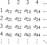 . This array contains every element of every
 ![]() , possibly with repetitions. We can list all entries by following the standard diagonal enumeration (zigzag through the array):
, possibly with repetitions. We can list all entries by following the standard diagonal enumeration (zigzag through the array):
![]()
![]() ,
, ![]()
![]() ,
, ![]() ,
, ![]()
![]() ,
, ![]() ,
, ![]()
…
This gives a sequence that eventually includes every pair (n,k), hence every element ![]() . Since there may be repetitions, the resulting list may have duplicates, but we can remove them (or map to the first occurrence). The resulting list is a countable enumeration of ∪ .Thus ∪ is countable (at worst countably infinite). QED
. Since there may be repetitions, the resulting list may have duplicates, but we can remove them (or map to the first occurrence). The resulting list is a countable enumeration of ∪ .Thus ∪ is countable (at worst countably infinite). QED
Theorem 14.77: The Cartesian product of two countable sets is countable.
Proof of Theorem 14.77: We prove this directly. Since A and B are countable, we can enumerate them ![]() and
and ![]() . Now consider the array of pairs
. Now consider the array of pairs
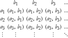 Again, use the diagonal enumeration:
This sequence eventually hits every pair ![]() . Thus A×B can be put into a countable list (with possible repetitions if A or B is finite, which can be removed). Therefore A×B is countable. QED
. Thus A×B can be put into a countable list (with possible repetitions if A or B is finite, which can be removed). Therefore A×B is countable. QED
Theorem 14.78 Cantor’s Theorem: For any set A, the power set P(A) is not equinumerous with A (there is no bijection between A and P(A)).
Proof of Theorem 14.78: We will prove this by contradiction. Suppose, for the sake of contradiction, that there does exist a bijection f:A→P(A). That is, every subset of A is hit by exactly one element of A, for every S⊆A, there is a unique a∈A such that f(a)=S. Now construct a special subset D⊆A (the “diagonal set”) as follows, D={x∈A∣x∉f(x)}. This is a perfectly well-defined subset of A, so D∈P(A). Since f is a bijection (hence surjective), there must exist some element b∈A such that f(b)=D. Now ask the key question, “Does b belong to D?”
Case 1: Suppose b∈D. By the definition of D, this means b∉f(b). But f(b)=D, so b∉D. This is a contradiction.
Case 2: Suppose b∉D. By the definition of D, this means it is not the case that b∉f(b), i.e., b∈f(b). But f(b)=D, so b∈D. This is also a contradiction.
In both cases we reach a contradiction. Therefore our initial assumption (that such a bijection f exists) must be false. Hence, there is no bijection from A to P(A). So A and P(A) are not equinumerous. QED
Theorem 14.79 Uncountability of the Reals: The set of real numbers R is uncountable (not equinumerous with N).
Proof of Theorem 14.79: We prove this by contradiction. Suppose, for the sake of contradiction, that R is countable. Then there exists a bijection f:N→R, so we can list all real numbers as an infinite sequence f(1), f(2), f(3), f(4), … .In particular, we can list all real numbers in the interval (0,1) ) (since if R were countable, any subset would also be countable). Write each number in its decimal expansion (avoiding infinite 9’s for uniqueness):
![]()
![]()
![]()
![]()
Now construct a new real number ![]() in (0,1) by the diagonal rule
in (0,1) by the diagonal rule
![]()
So x differs from f(k) in the k-th decimal place for every k. Therefore x≠f(k) for any k∈N. This means x is a real number in (0,1) that is not in the list {f(1),f(2),f(3),… }. But our assumption was that the list contained every real number in (0,1). This is a contradiction. Therefore the assumption that R is countable must be false. Hence R is uncountable—it is not equinumerous with N. QED
Exercise 14.58: Begin with Definition 14.106 and copy it into your notebook. Reflect on its meaning for a few minutes. Note any thoughts that come to mind. How would you explain this to someone sitting in front of you. Write this down. Then do this for each definition, principle, theorem, and proof.
Set Operations and Equinumerous Sets
By now you have seen that two sets can have exactly the same number of elements even if the elements themselves are completely different. We gave that idea a name: two sets are equinumerous (written A≈B or sometimes ∣![]() ) when there is a one-to-one correspondence (a perfect matching) between them. The surprising fact is that this “same-size” idea behaves extremely well when we start doing the usual set operations—union, intersection, difference, and so on. In other words, how we glue sets together or cut them apart does not depend on what the elements actually are, only on how many there are and how they overlap.
) when there is a one-to-one correspondence (a perfect matching) between them. The surprising fact is that this “same-size” idea behaves extremely well when we start doing the usual set operations—union, intersection, difference, and so on. In other words, how we glue sets together or cut them apart does not depend on what the elements actually are, only on how many there are and how they overlap.
Imagine two crates of spare parts on a spacecraft. Crate A has 27 bolts and Crate B has 19 nuts, and nothing is in both crates (the crates are completely separate). The total number of parts you have is obviously 27 + 19 = 46. Now suppose someone replaces every bolt with a washer and every nut with a rivet, but still keeps exactly 27 items in one crate and 19 in the other, with no overlap. You would still have 46 parts in total. The actual objects changed, but the counting did not. This simple counting fact turns into a theorem when we write it with sets
Theorem 14.80: Suppose A≈A' and B≈B', and the sets on each side have no elements in common, A∩B=Ø and A'∩B'=Ø. Then the combined sets also match in size, A∪B≈A'∪B'. In numbers, this says ∣![]() whenever the intersection is empty, and the same rule holds for the equinumerous copies.
whenever the intersection is empty, and the same rule holds for the equinumerous copies.
Proof of Theorem 14.80: We will prove this directly. Because A≈A' there is a perfect matching f:A→A'. Because B≈B' there is a perfect matching g:B→B'. Since A and B are disjoint, and A' and B' are disjoint, we can paste the two matchings together into a single function h:A∪B→A'∪B' defined by h(x)=f(x) if x∈A, h(x)=g(x) if x∈B. This h is a bijection, so A∪B≈A'∪B'. Done. This leads to a corollary, that is a theorem that extends from another theorem.
Corollary 14.1 Cardinality of a disjoint union: If A∩B=Ø, then ![]() .
.
The same formula holds for any sets that can be put into one-to-one correspondence with disjoint sets. This is exactly the counting rule you have used all your life when the boxes don’t overlap. The theorem tells us the rule survives even when we completely change what is inside the boxes, as long as we preserve the one-to-one matching and the “no overlap” condition. Later, when we meet infinite sets, you will see that this same theorem is what lets us say things like “the whole numbers and the even numbers have the same cardinality” even though one is a proper subset of the other.
Definitions
Definition 14.109 Disjoint union: The union of two disjoint sets A and B, often written A∪B when we want to emphasize disjointness.
Principles
Principle 14.53 Principle of Preservation under Set Operations: When we perform set operations (union, intersection, difference, etc.) on equinumerous sets, the cardinalities behave in a way that depends only on how the sets overlap or are combined, not on what the elements actually are.
Principle 14.54 Disjoint Union Principle: When two sets are disjoint, the size of their union is exactly the sum of their individual sizes.
Exercise 14.59: Begin with Definition 14.109 and copy it into your notebook. Reflect on its meaning for a few minutes. Note any thoughts that come to mind. How would you explain this to someone sitting in front of you. Write this down. Then do this for each definition, principle, theorem, and proof.
Exercise 14.60:
a) Two sets A and B are equinumerous, meaning there is a perfect one-to-one correspondence between their elements. Suppose ![]() .
.
1) If you form the union A ∪ B, what can you say about its size compared to ![]() ?
?
2) Why does the answer depend on whether A and B overlap?
(b) Let A and B be finite sets. You know ![]() and
and ![]() . Suppose
. Suppose ![]() .
.
1) What is ![]() ?
?
2) Explain the reasoning using the idea that overlapping elements get counted twice when you simply add the sizes.
c) Let A and B be equinumerous finite sets, so ![]() .
.
1) If A and B have no elements in common, what is ![]() ?
?
2) If A and B are the same set, what is ![]() ?
?
3) How does equinumerosity help you reason about these cases without listing every element?
d) In a physics experiment you have two collections of particles: set A with 8 particles and set B with 5 particles. Some particles belong to both collections (they are the same physical objects counted in different ways). Suppose 3 particles are in both A and B.
1) How many distinct particles are there in total?
2) Why is this a useful application of set operations in physics?
e) Let A be a finite set with ![]() . Let B ⊆ A with
. Let B ⊆ A with ![]() .
.
1) What is ![]() ?
?
2) If C is equinumerous to A \ B, what can you say about ![]() ?
?
3) Give a physical interpretation: suppose A is all possible states of a system and B is the states where energy exceeds a threshold.
f) You have learned that two sets are equinumerous if there is a bijection between them. Suppose A and B are equinumerous and finite.
1) Show that ![]() still holds.
still holds.
2) Why is this fact important when we later study infinite sets and cardinal numbers?
Cardinality
We now ask the most basic question about any set, “How big is it?” For finite sets the answer is easy—we simply count the elements, this tells us its cardinal number. For infinite sets, ordinary counting fails. We need a new idea that works for every set, finite or infinite.
The right idea is that two sets have the same size if we can pair every element of one with exactly one element of the other, with none left over. When such a perfect pairing exists, the sets are equinumerous, as we have explored in the previous sections. We already know that equinumerosity is an equivalence relation. Each equivalence class under this relation represents a possible “size.” As we have seen, we call these sizes cardinal numbers.
Definition 14.110 Cardinality: The cardinality of a set A, written |A| or ![]() , is the equivalence class of all sets that are equinumerous to A. In other words, |A| is the abstract size of A defined by the existence of a bijection.
, is the equivalence class of all sets that are equinumerous to A. In other words, |A| is the abstract size of A defined by the existence of a bijection.
We say two sets have the same cardinality, written ∣A∣=∣B∣, if and only if there exists a bijection between them.
We may now establish basic definitions for various classes of sets.
Definition 14.111 Finite Sets: A set is finite if it is equinumerous to some natural number n∈N. In this case we write ∣A∣=n, and we say A has n elements.
Every finite set can be put into one-to-one correspondence with a unique natural number. This gives us the familiar counting we learned as children.
Definition 14.112 Denumerable Sets: A set is denumerable (or countably infinite) if it is equinumerous to the set of all natural numbers N. We denote this cardinality by the Hebrew letter Aleph with a subscript of 0, we say, “Aleph-null.” ![]() .
.
Examples include the set of all integers Z, the set of all even numbers, and the set of all rational numbers Q. Each of these can be listed in an infinite sequence without missing any element or repeating any.
Definition 14.113 Uncountable Sets: A set is uncountable if it is infinite but not denumerable. Its cardinality is strictly larger than ![]() .
.
Its cardinality is written ![]() or c (the cardinality of the continuum, another name for the set of real numbers). Cantor proved that no bijection exists between N and R, so the cardinality of the reals is genuinely larger than any countable infinity.
or c (the cardinality of the continuum, another name for the set of real numbers). Cantor proved that no bijection exists between N and R, so the cardinality of the reals is genuinely larger than any countable infinity.
Definition 14.114 Ordering of Cardinal Numbers: We compare cardinal numbers using injections. For any two sets A and B,∣ thererr are three possible situations:
A∣≤∣B∣ means there exists an injection from A into B.
∣A∣=∣B∣ means there exists a bijection between A and B.
∣A∣<∣B∣ means ∣A∣≤∣B∣ but ∣A∣≠∣B∣ .
This ordering is very strict for infinite cardinals. We have the increasing sequence![]() .There are infinitely many distinct infinite cardinal numbers, each strictly larger than the previous.
.There are infinitely many distinct infinite cardinal numbers, each strictly larger than the previous.
So, what is the relevance of all of this abstract machinery in physics? In classical mechanics we constantly shift between discrete and continuous descriptions. The set of possible states labeled by integers is countable ![]() . The set of all possible positions or times is uncountable (
. The set of all possible positions or times is uncountable (![]() ). Understanding the difference between these sizes helps us see why some physical questions have countable answers while others require the full power of the continuum.
). Understanding the difference between these sizes helps us see why some physical questions have countable answers while others require the full power of the continuum.
Cardinal numbers give us a precise language for talking about “how many” when ordinary counting breaks down. They show that infinity comes in many different sizes, and that the real world seems to make essential use of the largest of these—the continuum.
Definitions
Definition 14.115 Aleph-null ![]() ): The cardinality of the natural numbers N. Every denumerable set has cardinality
): The cardinality of the natural numbers N. Every denumerable set has cardinality ![]() .
.
Definition 14.116 The Continuum: Another name for the set of real numbers R.
Definition 14.117 Cardinality of the continuum ![]() ): The cardinality of the real numbers R.
): The cardinality of the real numbers R.
Principles
Principle 14.55 Principle of Cardinality by Matching: Two sets have the same cardinality if and only if there exists a bijection between them. Size is determined solely by the existence of a perfect one-to-one correspondence.
Principle 14.56 Principle of Cardinal Ordering: Cardinal numbers are ordered by the existence of injections, ![]() means A can be injected into B.
means A can be injected into B.
Principle 14.57 Principle of Strict Hierarchy of Infinities: There is a strictly increasing sequence of infinite cardinalities ![]() .
.
Theorems
Theorem 14.81: The set of integers Z, the set of even numbers, and the set of rational numbers Q are all denumerable (have cardinality ![]() ).
).
Proof of Theorem 14.81: We show each set admits a bijection with the natural numbers N by a proof by cases.
Case 1. The integers Z are denumerable.
Define a function f:N→Z by f(n)={n/2if n is even,−(n+1)/2if n is odd}. Here are some examples, f(0)=0, f(1)=−1, f(2)=1, f(3)=−2, f(4)=2, f(5)=−3, … This is surjective since every integer appears. Positive integers appear at even indices, negative at odd, and 0 at n=0. This is injective since different values of n produce different values (even n give non-negative, odd n give negative, and the mapping is strictly increasing in absolute value). Thus f is a bijection, so ∣![]() .
.
Case 2. The even integers 2 Z are denumerable.
Define g:N→2Z by g(n)=2n. This is clearly injective (different n give different even numbers). It is surjective onto the evens because every even number 2k is hit by n = k. Thus g is a bijection, so ∣![]() .
.
Case 3. The rational numbers Q are denumerable.
We use the standard “diagonal argument” for positive rationals first, then extend to all rationals.
Step 3a: Positive rationals ![]() are denumerable.
are denumerable.
Consider the grid of fractions ![]() where p, q are positive integers. Arrange them in a table and traverse diagonally, skipping duplicates (non-reduced fractions):
where p, q are positive integers. Arrange them in a table and traverse diagonally, skipping duplicates (non-reduced fractions):
1/1
1/2, 2/1
3/1, 2/2 (skip), 1/3
1/4, 2/3, 3/2, 4/1
etc.
This enumeration hits every positive rational exactly once (after removing duplicates). Thus there is a bijection between N and ![]() , so
, so ![]() .
.
.Step 3b: All rationals Q are denumerable.
We can map the Even naturals → positive rationals (as above) and Odd naturals → negative rationals (similar diagonal), 0 → 0. More cleanly we can define a bijection by listing all rationals in a single sequence that includes negatives and zero, for example by ordering first by “height” |p| + |q| and then by sign. Since ![]() is countable and the negatives are also countable, their union with {0} is a countable union of countable sets, hence countable. Therefore
is countable and the negatives are also countable, their union with {0} is a countable union of countable sets, hence countable. Therefore ![]() .
.
Conclusion: All three sets admit bijections with N, so they all have cardinality ![]() . .QED
. .QED
Theorem 14.82 Basic Arithmetic of Cardinals: For infinite cardinals, ![]() ,
, ![]() , and
, and ![]() . (Adding or multiplying by finite numbers or even countably many copies does not increase the cardinality.)
. (Adding or multiplying by finite numbers or even countably many copies does not increase the cardinality.)
Proof of Theorem 14.82: We perform a proof by cases. All proofs rely on the fact that two sets have the same cardinality if there exists a bijection between them.
Case 1. ![]()
Given N (cardinality ![]() ). Consider the set N∪{∗}, where * is a new element not in N. Define a bijection f:N∪{∗}→N by f(∗)=0, f(n)=n+1for all n∈N. This is injective since different inputs go to different outputs. This is surjective since 0 is hit by *, and every k≥1 is hit by k−1. Thus there is a bijection between a set of cardinality
). Consider the set N∪{∗}, where * is a new element not in N. Define a bijection f:N∪{∗}→N by f(∗)=0, f(n)=n+1for all n∈N. This is injective since different inputs go to different outputs. This is surjective since 0 is hit by *, and every k≥1 is hit by k−1. Thus there is a bijection between a set of cardinality ![]() and N, so
and N, so ![]() .
.
Case 2. ![]()
Consider two disjoint copies of N, Let ![]() and
and ![]() . Their union has cardinality
. Their union has cardinality ![]() . Define a bijection
. Define a bijection ![]() by interleaving, g(n,1)=2n, g(n,2)=2n+1. This hits every even number with the first copy and every odd number with the second copy. It is clearly bijective. Therefore
by interleaving, g(n,1)=2n, g(n,2)=2n+1. This hits every even number with the first copy and every odd number with the second copy. It is clearly bijective. Therefore ![]() .
.
Case.3. ![]()
Consider the set N×N (all ordered pairs of natural numbers), which has cardinality ![]() .We can enumerate all pairs using the diagonal method where order pairs by the sum i+j, and within each sum go diagonally, (0,0) → (0,1), (1,0) → (0,2), (1,1), (2,0) → … . This gives a bijection with N (skip any duplicates if needed, but the standard diagonal enumeration covers everything exactly once when done properly). A simple explicit bijection is the Cantor pairing function: ⟨i,j⟩=(i+j)(i+j+1)2+j, which is a bijection from N×N to N. Thus
.We can enumerate all pairs using the diagonal method where order pairs by the sum i+j, and within each sum go diagonally, (0,0) → (0,1), (1,0) → (0,2), (1,1), (2,0) → … . This gives a bijection with N (skip any duplicates if needed, but the standard diagonal enumeration covers everything exactly once when done properly). A simple explicit bijection is the Cantor pairing function: ⟨i,j⟩=(i+j)(i+j+1)2+j, which is a bijection from N×N to N. Thus ![]() , so
, so ![]() . QED
. QED
Exercise 14.61: Begin with Definition 14.110 and copy it into your notebook. Reflect on its meaning for a few minutes. Note any thoughts that come to mind. How would you explain this to someone sitting in front of you. Write this down. Then do this for each definition, principle, theorem, and proof.
Properties of Finite Sets
Some sets are small enough that ordinary counting finishes in a reasonable time. We give those sets the special name of finite sets. We also collect the simple facts that always hold for them.
A set is finite when its elements can be paired perfectly with the numbers 1 through some natural number n, or with nothing at all if the set is empty.
The empty set has cardinality 0.
Theorem 14.83: Subsets of finite sets are finite. If A is finite and B ⊆ A, then B is finite and its cardinality is at most the cardinality of A.
Proof of Theorem 14.83: I will now introduce a new kind of proof called an idea-first proof. An idea-first proof begins with the core intuitive idea or physical insight, then translates that intuition into precise mathematical steps. It does not mean skipping rigor.
Start with the motivating idea (in plain language or with a picture).
Show why that idea leads naturally to the formal definitions or constructions.
Fill in all the necessary logical steps, definitions, and justifications.
End with a clear “therefore” that ties back to the original idea.
So, we will prove this theorem using an idea-first proof.
Since A is finite, we can list its elements: ![]() . The elements of B form some selection from that list. Simply cross off the items that do not belong to B. What remains is a list with at most n entries. Any list with at most n entries is finite. Thus B is finite. We now introduce the notion of a theorem that is used specifically to prove something, this is called a Lemma.
. The elements of B form some selection from that list. Simply cross off the items that do not belong to B. What remains is a list with at most n entries. Any list with at most n entries is finite. Thus B is finite. We now introduce the notion of a theorem that is used specifically to prove something, this is called a Lemma.
Lemma 14.1: Removing some elements from a nonempty finite set leaves a finite set. If A is finite and nonempty, and B ⊆ A, then A \ B is finite and |A \ B| = |A| − |B|.
Proof of Lemma 14.1: We prove this using an idea-first method. Start with the list of elements of A. Cross off every element that belongs to B. What is left is still an ordinary list, only shorter by exactly the number of elements you crossed off. A shorter list is still finite. QED
We then use this lemma to prove Theorem 14.83. QED
Theorem 14.84: For any two finite sets A and B, |A ∪ B| = |A| + |B| − |A ∩ B|.
Proof of Theorem 14.84: We prepare an idea-first proof. When you add |A| + |B|, every element that lies in both A and B gets counted twice. Subtract the overlap once. The result is the exact size of the union. QED
Theorem 14.85: The Cartesian product of two finite sets is finite. If A and B are finite, then A × B is finite and |A × B| = |A| ⋅ |B|.
Proof of Theorem 14.85: We prepare an idea-first proof. Imagine a rectangular table. Place the elements of A along the rows and the elements of B along the columns. Every ordered pair (a, b) occupies one cell. A table with m rows and n columns has exactly m ⋅ n cells.
Theorem 14.86: The power set of a finite set is finite. If A is finite and has n elements, then its power set 𝒫(A) is finite and ![]() .
.
Proof of Theorem 14.86: We produce an idea-first proof. For each element of A you face a simple yes-or-no choice: include it in the subset or leave it out. With n independent choices you obtain exactly ![]() possible subsets. This count includes the empty set (all choices “no”) and the full set A (all choices “yes”).
possible subsets. This count includes the empty set (all choices “no”) and the full set A (all choices “yes”).
Theorem 14.86 The Pigeonhole Principle: If you place more than n objects into n boxes, then at least one box must contain at least two objects. In set language, we write that if A and B are finite, |A| > |B|, and f: A → B is any function, then f is not injective. At least two distinct elements of A map to the same element of B.
Proof of Theorem 14.86: We produce an idea-first proof. Suppose every box held at most one object. Then you could fit at most |B| = n objects. But you are trying to place |A| > n objects. Therefore at least one box must hold two or more.
These facts about finite sets are reliable and useful. They rest on nothing more than careful counting and the idea of one-to-one matching. We use them constantly in physics without thinking, yet they are surprisingly powerful once we see where they come from.
Terms
Term 14.21 Small Set: A set whose elements can be counted in a reasonable (finite) amount of time.
Principles
Principle 14.58 Principle of Finite Counting: A finite set has a definite, fixed number of elements that can be reached by ordinary counting.
Principle 14.59 Principle of Subset Size: Any subset of a finite set is itself finite, and its size is at most the size of the original set.
Principle 14.60 Principle of Inclusion-Exclusion: When combining two finite sets, the size of their union is the sum of their sizes minus the size of their overlap.
Principle 14.61 Principle of Product Size: The Cartesian product of two finite sets has size equal to the product of their individual sizes.
Principle 14.62 Principle of Power Set Size: The power set of a finite set with n elements has exactly ![]() elements.
elements.
Exercise 14.62: Begin with Theorem 14.83 and copy it into your notebook. Reflect on its meaning for a few minutes. Note any thoughts that come to mind. How would you explain this to someone sitting in front of you. Write this down. Then do this for each ter, principle, theorem, lemma, and proof.
Exercise 14.63:
a) A laboratory has 12 sensors. Each sensor can be either working or broken.
1) How many possible subsets of working sensors are there?
2) Explain why your answer follows from the idea that each sensor gives an independent yes/no choice.
(b) Let ( be a finite set with 7 elements. Let B be a subset of A with 4 elements.
1) Is B finite?
2) What is the largest possible size of A \ B?
3) What is the smallest possible size of A \ B?
Use the idea of crossing items off a list to explain your answer.
c) Suppose set A has 9 elements and set B has 6 elements. The two sets share 3 elements.
1) What is the size of A ∪ B?
2) Why does the overlapping part get subtracted in the calculation?
d) A system has 4 possible positions and 3 possible velocities.
1) How many possible (position, velocity) pairs are there?
2) Why is this number the size of the Cartesian product of the two sets?
e) A set C has 4 elements.
1) How many subsets does C have?
2) How many of those subsets contain exactly 2 elements?
3) Explain why the total number is a power of 2 using the yes/no choice idea.
f) There are 13 astronauts and only 8 seats on a shuttle.
1) Use the pigeonhole principle to explain why at least one seat must be occupied by more than one astronaut? No — wait, that’s not right. Actually: Use the pigeonhole principle to explain why it is impossible for every astronaut to have a unique seat.
2) Give a physics analogy: suppose you have 13 possible energy states and only 8 detectors. What must happen?
Denumerable Sets
Some sets go on forever. Yet we can still list every element in a single infinite sequence without skipping any or repeating any. Sets that allow such a perfect infinite list have a very special kind of infinity. A set is denumerable (also called countably infinite) when its elements can be arranged in one infinite list that contains every element exactly once. Formally, a set is denumerable if there exists a bijection between the set and the natural numbers N. We write the cardinality of every denumerable set as ![]() (read “aleph-null”).
(read “aleph-null”).
Examples you already know include:the natural numbers N themselves, the integers Z, and the even numbers. All three are denumerable, even though one is a proper subset of another.
Theorem 14.87: Every infinite subset of a denumerable set is itself denumerable.
Proof of Theorem 14.87: We produce an idea-first proof. Start with the infinite list of the bigger denumerable set, ![]() Walk down this list and keep only the elements that belong to the subset. You may skip some entries, but because the subset is infinite you never run out of elements, and you never repeat any. The result is a new infinite list with no gaps and no duplicates. Therefore the subset is denumerable. QED
Walk down this list and keep only the elements that belong to the subset. You may skip some entries, but because the subset is infinite you never run out of elements, and you never repeat any. The result is a new infinite list with no gaps and no duplicates. Therefore the subset is denumerable. QED
Corollary 14.3: Every subset of a countable set (finite or denumerable) is countable.
Proof of Corollary 14.3: We build a proof by cases. Let A be a countable set, and let B⊆A. We consider two cases.
Case 1: A is finite.
If A has n elements, then by theorem 14.87, any subset B of A is also finite. Thus B is countable.
Case 2: A is denumerable.
Since A is denumerable, there exists a bijection f:N→A. That is, we can list the elements of A as an infinite sequence without repetition, ![]() , where
, where ![]() . Now consider the subset B⊆A. We construct a list for B by walking through the sequence of A and keeping only the elements that belong to B .Because B may be finite or infinite, we have two sub-cases, but the argument is the same in spirit. If B is finite, we are done—it is countable.
. Now consider the subset B⊆A. We construct a list for B by walking through the sequence of A and keeping only the elements that belong to B .Because B may be finite or infinite, we have two sub-cases, but the argument is the same in spirit. If B is finite, we are done—it is countable.
If B is infinite, then as we walk down the infinite list of A, we will encounter infinitely many elements that belong to B (since B is infinite). We can therefore create a new sequence by recording only those elements of A that are in B, in the order they first appear. This new sequence contains every element of B exactly once and never ends. Hence it is a bijection with N, so B is denumerable.
In both sub-cases, B is countable.
Conclusion: Whether A is finite or denumerable, every subset B⊆A is countable. QED
Theorem 14.88: The Cartesian product N×N is denumerable.
Proof of Theorem 14.88: We build an idea-first proof including an explicit bijection. Picture the infinite grid of all ordered pairs (m, n) where m and n are natural numbers. Travel along the anti-diagonals:
(1,1)
(1,2), (2,1)
(1,3), (2,2), (3,1)
(1,4), (2,3), (3,2), (4,1)
…
Each anti-diagonal has a finite number of pairs, and every pair eventually appears on some anti-diagonal. Thus the entire infinite grid can be listed in one single infinite sequence. QED
Corollary 14.4: The Cartesian product of any finite number of denumerable sets is denumerable.
Proof of Corollary 14.4: We use a proof by induction. We already know that the product of two denumerable sets N×N is denumerable by Theorem 14.88. We now extend this to any finite number of factors by induction on the number of sets.
Base case (two sets):
We have already shown that N×N is denumerable.
Inductive step: Assume the statement holds for k denumerable sets: the product N×N×···×N (k times) is denumerable. Now consider k+1 denumerable sets. Let ![]() each be denumerable. We can group them as
each be denumerable. We can group them as ![]() .
.
By the induction hypothesis, the product of the first k sets is denumerable—call it D. So we have ![]() , where both D and
, where both D and ![]() are denumerable. By Theorem 14.88,
are denumerable. By Theorem 14.88, ![]() is denumerable.
is denumerable.
Therefore, by induction, the Cartesian product of any finite number of denumerable sets is denumerable. QED
Theorem 14.89: The set of rational numbers Q is denumerable.
Proof of 14.89: We use an idea-first proof. Every rational number can be written (in lowest terms) as p/q with p an integer and q a positive integer. We can list all such fractions using the same diagonal trick on the grid of pairs, after handling signs and skipping duplicates. Duplicates do not hurt—we only need one infinite list that eventually includes every rational. Since Q injects into Z×N and the latter is denumerable, Q is at most denumerable. Since Q is infinite, it is exactly denumerable. QED
Theorem 14.90: The union of a denumerable family of denumerable sets is denumerable.
Proof of Theorem 14.90: We build an idea-first proof. Let ![]() be the family of sets. Each
be the family of sets. Each ![]() has its own infinite list. Arrange all these lists into an infinite array. Now walk along the anti-diagonals of this big array. Every element of every
has its own infinite list. Arrange all these lists into an infinite array. Now walk along the anti-diagonals of this big array. Every element of every ![]() appears somewhere in the array, so the entire union appears in one infinite sequence. QED
appears somewhere in the array, so the entire union appears in one infinite sequence. QED
Corollary 14.5: The intersection of any finite or denumerable family of countable sets is countable. (Intersection can only make a set smaller, and every subset of a countable set is countable.)
Proof of Corollary 14.5: We prove this directly by cases with element-chasing. Let ![]() be a family of countable sets, where the index set is either finite or denumerable (i.e., the family has at most countably many members). We want to show that the intersection
be a family of countable sets, where the index set is either finite or denumerable (i.e., the family has at most countably many members). We want to show that the intersection ![]() is countable.
is countable.
Case 1: The family is finite.
Suppose there are only finitely many sets, say ![]() . The intersection
. The intersection ![]() is a subset of
is a subset of ![]() (for example). Since
(for example). Since ![]() is countable, and we already know that every subset of a countable set is countable by Corollary 14.3, it follows immediately that
is countable, and we already know that every subset of a countable set is countable by Corollary 14.3, it follows immediately that ![]() is countable.
is countable.
Case 2: The family is denumerable.
Now suppose the family is countably infinite: ![]() . Again, the intersection
. Again, the intersection ![]() is a subset of
is a subset of ![]() . Since
. Since ![]() is countable, and every subset of a countable set is countable, the intersection is countable.
is countable, and every subset of a countable set is countable, the intersection is countable.
Conclusion: In both cases—whether the family is finite or denumerable—the intersection is a subset of one of the countable sets in the family. Therefore the intersection is countable. QED
Theorem 14.91: Every infinite set contains a denumerable subset.
Proof of Theorem 14.91: We provide an idea-first proof. Because the set is infinite, pick any element ![]() . Remove
. Remove ![]() ; the remainder is still infinite, so pick
; the remainder is still infinite, so pick ![]() different from
different from ![]() . Continue forever. The process never stops, and all chosen elements are distinct by construction. The set
. Continue forever. The process never stops, and all chosen elements are distinct by construction. The set ![]() is denumerable and sits inside the original infinite set. QED
is denumerable and sits inside the original infinite set. QED
These theorems are the workhorses that let us say “the integers are no bigger than the naturals,” “all rational numbers fit on a single infinite list.1,”
They are also the last calm shore before we meet the uncountable sets, where these nice listing tricks suddenly fail.
Terms
Term 14.21 Infinite list: A sequence that goes on forever without end, yet contains every element of the set exactly once.
Definitions
Definition 14.118 Denumerable set (also called countably infinite set): A set whose elements can be arranged in a single infinite list that contains every element exactly once. Formally we state that a set A is denumerable if there exists a bijection between A and the natural numbers N. These have cardinality ![]() The cardinality shared by every denumerable set. We write
The cardinality shared by every denumerable set. We write ![]() when A is denumerable.
when A is denumerable.
Principles
Principle 14.63 Principle of Countable Listing: A set is denumerable when we can list its elements in one infinite sequence without skipping any or repeating any.
Principle 14.64 Principle of Subset Inheritance: Every subset of a denumerable set is either finite or denumerable (hence countable).
Principle 14.65 Principle of Diagonal Enumeration: The Cartesian product of two denumerable sets can be listed by traveling along the anti-diagonals of the infinite grid of pairs.
Principle 14.66 Principle of Countable Unions: The union of a denumerable family of denumerable sets is itself denumerable.
Principle 14.67 Principle of Countable Subsets: Every infinite set contains at least one denumerable subset.
Exercise 14.64: Begin with Theorem 14.87 and copy it into your notebook. Reflect on its meaning for a few minutes. Note any thoughts that come to mind. How would you explain this to someone sitting in front of you. Write this down. Then do this for each term, definition, principle, theorem, lemma, corollary, and proof.
Exercise 14.65:
a) Some sets go on forever, yet we can still list every element in a single infinite sequence without skipping or repeating any.
1) What name do we give to such sets?
2) Why is this property important when we study infinite sets?
b) The set of all integers Z is denumerable.
1) Give an explicit infinite list that contains every integer exactly once.
2) Explain why your list shows that ![]() .
.
c) The set of even integers is a proper subset of the integers.
1) Show that the even integers are denumerable by giving a bijection with N.
2) Does this contradict the idea that a proper subset should be smaller? Explain.
d) We know N×N is denumerable.
1) Describe in your own words how the diagonal argument lists all ordered pairs (m, n).
2) Why does this show that the Cartesian product of two denumerable sets is still denumerable?
e) The set of rational numbers Q is denumerable.
1) Explain why we can list all positive rationals using the same diagonal trick as for N×N.
2) How do we extend this to include negative rationals and zero?
f) In physics we often deal with countable collections of states (for example, energy levels labeled by integers).
1) Why is it useful that the set of all such labeled states is denumerable?
2) Give one example from physics where a denumerable set appears naturally.
Uncountable Sets
Some infinities are so large that no list—no matter how long—can ever contain all of their elements. These sets are simply too big to count, even with an infinite amount of time.
A set is uncountable if it is infinite and no bijection exists between it and the natural numbers N. In other words, every attempt to list its elements will always miss infinitely many of them.
Theorem 14.92 Cantor’s Diagonal Argument: The open interval (0,1) is uncountable.
Proof of Theorem 14.92: We produce an idea-first proof. Suppose, for the sake of contradiction, that (0,1) is countable. Then its elements can be listed as an infinite sequence of decimals:
![]()
![]()
![]()
where each ![]() is a digit from 0 to 9. Now construct a new number
is a digit from 0 to 9. Now construct a new number ![]() by choosing each digit
by choosing each digit ![]() as follows,
as follows,
If ![]() , let
, let ![]() .
. ![]() , let
, let ![]() .
.
The number x lies in (0,1), yet it differs from ![]() in the first decimal place, from
in the first decimal place, from ![]() in the second place, from
in the second place, from ![]() in the third place, and so on. Therefore x is not anywhere on the list. This leads to a contradiction.
in the third place, and so on. Therefore x is not anywhere on the list. This leads to a contradiction.
Hence no such list can exist, and (0,1) is uncountable. QED
Theorem 14.93: The set of all real numbers R is uncountable.
Proof of Theorem 14.93: We produce an idea-first proof. The interval (0,1) is a subset of R, and we just showed (0,1) is uncountable. A set that contains an uncountable subset must itself be uncountable (because if R were countable, every one of its subsets would also be countable). The cardinality of the real numbers R (and of any interval (a,b) with a < b) is called the cardinality of the continuum and is denoted ![]() or simply c. We know
or simply c. We know ![]() because N injects into R but no bijection exists. QED
because N injects into R but no bijection exists. QED
Theorem 14.94: The set of irrational numbers R \ Q is uncountable (and has cardinality ![]() ).
).
Proof of Theorem 14.94: We produce an idea-first proof. We already know ![]() and |Q| = ℵ₀. If the irrationals were countable, then R = (R \ Q) ∪ Q would be the union of two countable sets, hence countable. But R is uncountable, so the irrationals must be uncountable. In fact, removing the countable set Q does not change the cardinality
and |Q| = ℵ₀. If the irrationals were countable, then R = (R \ Q) ∪ Q would be the union of two countable sets, hence countable. But R is uncountable, so the irrationals must be uncountable. In fact, removing the countable set Q does not change the cardinality ![]() . QED
. QED
Theorem 14.95: The Cartesian product (0,1] × (0,1] has the same cardinality as (0,1].
Proof of Theorem 14.95: We produce an idea-first proof. First, (0,1] has cardinality ![]() because it differs from (0,1) by only one point. Now we show
because it differs from (0,1) by only one point. Now we show ![]() . One direction is easy, the function f(x,y) = x is an injection from (0,1] × (0,1] into (0,1], so the cardinality is at most
. One direction is easy, the function f(x,y) = x is an injection from (0,1] × (0,1] into (0,1], so the cardinality is at most ![]() . For the other direction, map (0,1] into the square by interleaving decimal digits (or use any of several standard bijections). A simple geometric way is to take any number z ∈ (0,1] and split its decimal expansion into the even- and odd-placed digits to produce two numbers in (0,1]. This gives an injection from (0,1] into (0,1] × (0,1], proving the square is at least as large as the interval.
. For the other direction, map (0,1] into the square by interleaving decimal digits (or use any of several standard bijections). A simple geometric way is to take any number z ∈ (0,1] and split its decimal expansion into the even- and odd-placed digits to produce two numbers in (0,1]. This gives an injection from (0,1] into (0,1] × (0,1], proving the square is at least as large as the interval.
Since the two sets squeeze the same cardinality from above and below, ![]() .(The same argument works for R × R, the entire plane, or even
.(The same argument works for R × R, the entire plane, or even ![]() for any finite n.) This is the first shocking sign of how huge the continuum really is: a single open interval already contains as many points as the whole infinite plane!
for any finite n.) This is the first shocking sign of how huge the continuum really is: a single open interval already contains as many points as the whole infinite plane!
Terms
Term 14.22 Too big to list: The intuitive sense that some infinite sets cannot be arranged in any single infinite sequence without missing infinitely many elements.
Definitions
Definition 14.119 Uncountable set: An infinite set that is not denumerable. That is, no bijection exists between the set and the natural numbers N.
Definition 14.120 Cardinal inequality: ∣A∣<∣B∣ means there is an injection from A into ( B ), but no bijection between them.
Principles
Principle 14.68 Principle of Uncountability: A set is uncountable if every possible attempt to list its elements in an infinite sequence must leave out infinitely many elements.
Principle 14.69 Principle of Subset Inheritance for Uncountability: If a set contains an uncountable subset, then the whole set is uncountable.
Principle 14.70 Principle of Continuum Size: The real numbers R have cardinality ![]() , which is strictly larger than
, which is strictly larger than ![]() .
.
Principle 14.71 Principle of Diagonal Construction: One powerful way to prove uncountability is to assume a list exists and then construct a new element that cannot appear anywhere on that list (Cantor’s diagonal argument).
Exercise 14.66: Begin with Theorem 14.92 and copy it into your notebook. Reflect on its meaning for a few minutes. Note any thoughts that come to mind. How would you explain this to someone sitting in front of you. Write this down. Then do this for each term, definition, principle, theorem, and proof.
Exercise 14.65:
a) In a single sentence, explain why Cantor’s diagonal number cannot appear in the supposed list.
b) Why does removing the single point {0} from [0,1) not change its cardinality?
c) True or false: every subset of R is either countable or has cardinality ![]() . (No proof needed yet—just intuition.)
. (No proof needed yet—just intuition.)
d) Explain in your own words why the set of all real solutions to polynomial equations with integer coefficients must be countable.
More About Cardinal Numbers
Two big questions now sit in front of us. They feel almost philosophical until we turn them into precise mathematics.
Question 1: If a set is infinite, must there be another infinite set that is strictly larger than the first one?
Question 2: When we have any two sets A and B, is it always true that either |A| ≤ |B| or |B| ≤ |A|? In other words, can every pair of cardinal numbers be compared with a clear “smaller,” “equal,” or “larger”?
The answers turn out to be “yes” to the first question and “yes” to the second (with some care).
The proofs are surprisingly deep.
Theorem 14.96 Cantor’s 1891 Theorem: No set is equinumerous with its own power set. For every set A, |A| < |𝒫(A)|.
Proof of Theorem 14.96: This will be an idea-first proof with a diagonal argument. First, |A| ≤ |𝒫(A)| is easily obtained. Send each element a ∈ A to the singleton {a} ∈ 𝒫(A). This is an injection. Now suppose, for the sake of contradiction, there is a bijection f: A → 𝒫(A). Consider the “diagonal set” D = { x ∈ A | x ∉ f(x) }. D is definitely a subset of A, so D = f(t) for some t ∈ A. Is t ∈ D? If t ∈ D, then by the definition of D we must have t ∉ f(t), so t ∉ D this is a contradiction. If t ∉ D, then t satisfies the condition for membership in D, so t ∈ D a contradiction again. Therefore no such bijection f can exist. Hence |A| < |𝒫(A)| strictly.
This theorem immediately answers Question 1. Starting from any infinite set, take its power set (strictly bigger), then the power set of that (even bigger), and so on. There is no “largest” infinity.
Theorem 14.97 The Cantor–Bernstein Theorem (Schröder–Bernstein theorem): If there is an injection from A to B and an injection from B to A, then there is a bijection between A and B. We write, if |A| ≤ |B| and |B| ≤ |A|, then |A| = |B|.
Proof of Theorem 14.97: We will produce an idea-first proof. Assume we have injections f: A → B and g: B → A. Some points in A may be “hit” by g and some may not. Follow the chains backward starting with any element in A that is not in the image of g, then follow it forward with f, backward with g, forward with f, and so on. These chains are either infinite in both directions, infinite only forward, or end after a finite number of steps. We can explicitly pair up elements along these chains in a way that respects both injections, and everything left over gets matched directly. The result is a bijection between A and B. QED
Cantor–Bernstein is the tool that lets us say things like R∼R×R or (0,1)∼R with complete confidence once we have injections both ways.
With the tools now in hand—injections define ≤, Cantor–Bernstein lets us conclude equality when ≤ holds both ways, and the power-set theorem guarantees strictly larger cardinals—we can say that every pair of sets satisfies exactly one of |A| < |B|, |A| = |B|, or |A| > |B|. (Proving this for arbitrary sets requires the Axiom of Choice or equivalent principles, but for most sets we meet in physics and ordinary mathematics it is perfectly safe.)
Quick Picture of the Cardinal Landscape
0, 1, 2, … (finite)
↓![]() (denumerable)
(denumerable)
↓![]() or c (continuum)
or c (continuum)
↓![]() ,
, ![]() , , … (power set tower—the strictly increasing sequence obtained by repeatedly taking power sets)
, , … (power set tower—the strictly increasing sequence obtained by repeatedly taking power sets)
↓![]() ,
, ![]() , … (higher alephs)
, … (higher alephs)
Each arrow means “strictly smaller than the next.”
There is no largest cardinal, and between any two there is always room for infinitely many more.
These two theorems—power-set strict growth and Cantor–Bernstein—are the crown jewels of basic cardinal arithmetic. With them in your toolbox, you can now compare any two infinities you are likely to meet in physics, confidently and correctly.
Exercise 14.68: Begin with Theorem 14.96 and copy it into your notebook. Reflect on its meaning for a few minutes. Note any thoughts that come to mind. How would you explain this to someone sitting in front of you. Write this down. Then do this for each theorem, and proof.
Exercise 14.69:
a) We now know that some infinities are larger than others.
1) Why does Cantor’s theorem tell us there is no “largest” infinity?
2) Give one example from the section that shows how taking the power set always produces a strictly bigger set.
b) Let A be any set.
1) Explain in your own words why |A| < |𝒫(A)| using the diagonal idea.
2) Why does this theorem immediately answer the question “If a set is infinite, must there be a strictly larger infinite set?”
c) Suppose we have two sets A and B such that there is an injection from A into B and an injection from B into A.
1) What does the Cantor–Bernstein theorem conclude?
2) Why is this theorem useful when we cannot directly find a bijection but can show injections both ways?
d) We have the cardinal numbers ![]() and
and ![]() .
.
1) Which one is larger?
2) Explain why ![]() using the fact that the reals are uncountable.
using the fact that the reals are uncountable.
e) Start with the natural numbers, which have cardinality ![]() .
.
1) What is the cardinality of its power set?
2) What is the cardinality of the power set of that power set?
3) Describe the beginning of the “power set tower” and explain why it goes on forever.
f) In classical mechanics we often deal with the continuum of possible positions or times.
1) Why is it important to know that the cardinality of the real numbers is ![]() ?
?
2) Give one example from physics where the distinction between countable and uncountable infinities matters.
The Axiom of Choice
In the previous section we asked two big questions about infinite sets:Is there always a strictly larger infinity? (Yes – answered by the power-set theorem.) Can every pair of sets be compared – does one always have cardinality less than or equal to the other?
We now settle the second question completely, but the answer needs a new axiom.
Axiom 14.18 The Axiom of Choice (AC): When you are given a collection of non-empty sets (even infinitely many of them), it is possible to pick one element from each set, all at once. Formal;y we write that for any family of non-empty sets ![]() (I can be infinite), there exists a choice function
(I can be infinite), there exists a choice function ![]() such that
such that ![]() for every i ∈ I. In everyday language: even if there are infinitely many boxes, each containing at least one marble, you can pick exactly one marble from each box simultaneously.
for every i ∈ I. In everyday language: even if there are infinitely many boxes, each containing at least one marble, you can pick exactly one marble from each box simultaneously.
This sounds harmless, almost obvious, yet it cannot be proved from the other standard axioms of set theory. It must be assumed separately.
Axiom 14.19 Zorn’s Lemma (one of the most useful forms of AC) If a partially ordered set has the property that every chain (every totally ordered subset) has an upper bound, then the whole set has at least one maximal element.
With the Axiom of Choice (or any of its equivalents), every pair of sets can be compared:
Theorem 14.98: For any two sets A and B, exactly one of the following holds: |A| < |B|, |A| = |B|, or |A| > |B|. In other words, the cardinal numbers are totally ordered.
Proof of Theorem 14.98: We produce an idea-first proof. Using AC we can well-order every set (line its elements up so that every non-empty subset has a least element). Once two sets are well-ordered, we can compare their order-types directly where the “shorter” well-ordering injects into the longer one, and Cantor–Bernstein finishes the job. Without AC, comparability can fail in very pathological models of set theory, but for all practical purposes in mathematics and physics, we accept AC and enjoy total comparability. QED
Theorem 14.99: Every infinite set contains a denumerable subset.
Proof of Theorem 14.99: We develop an idea-first proof (now using AC). Let S be infinite. Using the Axiom of Choice, pick an element ![]() .
.![]() is still infinite, so pick
is still infinite, so pick ![]() . Continue: at step n pick
. Continue: at step n pick ![]() from the remaining infinite set. The function
from the remaining infinite set. The function ![]() is injective (all
is injective (all ![]() distinct), and its image
distinct), and its image ![]() is a denumerable subset of S. (Note: earlier we proved this without AC by constructing the sequence explicitly, but the AC version is the one that works even for completely wild sets that have no obvious structure.)
is a denumerable subset of S. (Note: earlier we proved this without AC by constructing the sequence explicitly, but the AC version is the one that works even for completely wild sets that have no obvious structure.)
Most working mathematicians and physicists treat the Axiom of Choice as true because the alternative leads to extremely strange and unusable universes.
Terms
Term 14.22 Choice: The intuitive act of picking one element from each set in a collection, even when the collection is infinite.
Definitions
Definition 14.121 Choice function: A function that selects exactly one element from each non-empty set in a given family.
Principles
Principle 14.72 Principle of Equivalence: The Axiom of Choice is logically equivalent to Zorn’s Lemma and to the Well-Ordering Principle (assuming the other axioms of ZF set theory).
Principle 14.73 Principle of Cardinal Comparability: With the Axiom of Choice, every pair of sets can be compared: for any two sets A and B, exactly one of |A| < |B|, |A| = |B|, or |A| > |B| holds.
Summary
Write a summery of this chapter.
For Further Study
Douglas Smith, Maurice Eggen, Richard St. Andre, (2014), A Transition to Advanced Mathematics. Cengage Learning 8th Edition. This is a very nice presentation of this material. It covers a lot of the material of this chapter.
Steven Galovich, (1989), Introduction to Mathematical Structures. Harcourt Brace Janovich Publishers and Its Subsidiary, Academic Press. This is my favorite book on the subject of this lesson.
Introduction to Proofs (Khan Academy) Link: https://www.khanacademy.org/math/geometry/hs-geo-foundations/hs-geo-proof-foundations/v/introduction-to-proof . Duration: 10 minutes. Starts with basic proof strategies (direct proof, contradiction), with examples and interactive elements.
Set Theory | All-in-One Video by Will Wood (highly recommended starting point)
→ Excellent overview of sets, subsets, power sets, relations, functions, cardinality, countable vs uncountable, and Cantor’s diagonal argument.
Link: https://www.youtube.com/watch?v=5ZhNmKb-dqk
Everything You Need To Know About Set Theory by BrainStation
→ Covers basics through advanced topics including finite/infinite sets, cardinality, and some logic. Good for beginners.
Link: https://www.youtube.com/watch?v=iTZfATpm0Yk
Cantor, sets, diagonal proof, continuum and cardinality by Vladan Djordjevic
Clear explanation of diagonal argument and why the reals are uncountable.
Link: https://www.youtube.com/watch?v=nzKlGgjqGns
Cantor’s Diagonal Argument: The rationals and reals have different sizes?! by jHan
Fun and intuitive take on why rationals are countable but reals are not.
Link: https://www.youtube.com/watch?v=0HF39OWyl54
Set Theory 1.2: Ordinals by Fematika
Excellent introduction to von Neumann ordinals/natural numbers and how they satisfy Peano axioms.
Link: https://www.youtube.com/watch?v=Ug6Je_ah58U
Equivalence Relations and Partial Orders by KindiakMath
Good visual explanations with examples.
Link: https://www.youtube.com/watch?v=ORVejvMgcL4
Equivalence Relations, Partial Orders and Hasse Diagrams by Stephen Woodcock
Clear and concise with diagrams.
Link: https://www.youtube.com/watch?v=6qA7tws-zsA