Lesson 13 Physical Quantities and Units

“If you cannot measure it, you cannot improve it.” Lord Kelvin

“To measure is to know.” James Clerk Maxwell

Introduction

With geometry as the language of space, we now turn to the language of measurement. The properties of the physical world that we can assign numbers to are physical quantities. The standards we use to compare these quantities are units.

The process of describing the universe begins with measuring. The ability to express a length, time, or force numerically gives us the power to predict, test, and understand. The system of units that unifies these measurements worldwide is the International System of Units (SI). It is not the only system.

The skill of moving between different units is unit conversion. The consistency of equations across units is dimensional homogeneity. The method that uses dimensions to derive relationships is dimensional analysis.

The theorem that tells us how many dimensionless groups govern a physical system is the Buckingham Pi Theorem. The problems that estimate answers with minimal data are Fermi problems. The quick calculations that guide intuition are back-of-the-envelope calculations.

The study of how errors accumulate to affect results is error propagation. The design of experiments to minimize uncertainty is experiment design. The patterns that emerge when systems scale are scaling laws.

In this lesson, we learn to measure, convert, analyze, and estimate—tools that turn observation into knowledge.

Physical Quantities

We now turn to the study of the measurable features of the physical world. The properties of nature that we can assign numbers to are physical quantities.

The idea that a car moves at 60 kilometers per hour, that a light bulb uses 100 joules of energy, or that a spring stretches 2 centimeters under a 5-Newton force captures the essence of measurement. The process of assigning a number and a unit to a property is quantification.

The attributes of objects or systems that change or remain constant are physical variables. The relationship between a change in one variable and a change in another is a physical relationship.

The distinction between constant and changing variables separates static from dynamic systems.

The connection between distance and time gives speed. The connection between force and mass gives acceleration. The connection between work and distance gives energy.

These ideas—magnitude, change, relationship—form the foundation of physics. The words—mass, speed, acceleration, energy—are labels we attach to them.

Undefined Terms

Term 13.1 Physical Quantity: A property that can be measured.

Term 13.2 Change: The variation (or constancy) in a quantity over space, time, or conditions.

Formal Definitions

Definition 13.1 Physical Quantity: A property of nature that can be assigned a numerical value through measurement (i.e., quantified).

Definition 13.2 Measurement: Assigning a number along with a unit to a property.

Definition 13.3 Physical Variable: An attribute that can change or stay constant.

Definition 13.4 Physical Relationship: How one variable affects another.

Definition 13.5 Quantification: The act of measuring.

Axioms

Axiom 13.1: The physical world contains properties that can be reliably assigned numbers via measurement, allowing prediction, testing, and understanding.

Axiom 13.2: The laws of physics are independent of the choice of units; only the relationships between quantities matter.

Axiom 13.3: Physical relationships arise from connections between magnitudes and changes in variables/

Exercise 13.1: Begin with Term 13.1 and copy it into your notebook. Reflect on its meaning for a few minutes. Note any thoughts that come to mind. How would you explain this to someone sitting in front of you. Write this down. Then do this for each term, definition, and axiom.

Units

With physical quantities as the measurable properties of nature, we now turn to the standards we use to express them. The reference standard that allows us to compare one quantity to another is a unit.

The idea that 5 meters is longer than 3 meters, or that 2 kilograms is heavier than 1 kilogram, rests on the comparison made possible by units. The process of assigning a unit to a quantity is calibration.

The variables that remain unchanged when the size of the system changes are intensive variables (for example temperature and density). The variables that grow proportionally with the size of the system are extensive variables (for example mass and volume). The variables that count discrete objects are discrete variables (for example, the number of particles or number of steps).

The meaning we attach to a quantity can be expressed by a unit (for example the meter or the second) or by a concept (for example the length or  time). The distinction between direct measurement (say using a ruler) and indirect measurement (calculating speed from distance and time) separates primary from secondary data.

The units that arise from fundamental standards are substantial units (for example the meter or the kilogram). The units that emerge from natural phenomena are natural units (for example the light-year or the atomic mass unit). The units that cannot be expressed in terms of others are basic units; those built from basic units are derived units.

The relationship among units reflects the physical relationship among quantities: 1 joule = 1 newton · meter. The mathematical interpretation of a physical variable treats it as a number multiplied by a unit: v = 5 m .

The requirement that language about units be consistent is linguistic soundness. The reason we can treat physical variables mathematically is that units cancel in equations, leaving pure numbers.

The mathematical relationship among units is multiplication and division: speed = distance / time. The statements that express physical laws are physical equations (for example, F = m a).

The variables that describe natural phenomena without artificial scales are natural variables (for example, the speed of light). The process of building a coherent set of units is constructing a system of units. The choice of which quantities to take as basic is the selection of units in a system. The units that exist outside any system are units outside of systems (for example, the furlong or the stone).

The measures of plane angles are degrees and radians. We have already seen the degree. If we divide the degree by 60 we have the minute of angle, denoted by ‘. If we divide the minute of angle by 60 we have the second of arc, denoted ”.

In physics we do not generally use the degree as a measure of angle. Instead we use something that we call the radian; we say that there are 2 π radians in 360°, or 1radian=π/180°, thus 90°=π/2 radians, and 30°=π/6 radians. Thus a radian is about 57°.

Speaking of a unit without specifying the system of the unit allows us to generalize that unit. For example, if we speak of a generic length we would refer to a generic unit of length. Instead of writing generic unit of whatever, we call it a dimension of whatever. We denote a dimension by surrounding the variable label by square brackets. For example, the dimension of length is denoted [L]. The meaning of dimensions is the type of quantity (length, time, mass), independent of specific units.

These ideas—standard, comparison, relationship, dimension—form the language of measurement. The words—meter, second, joule, [L], [T]—are labels we attach to them.

Undefined Terms

Term 13.3 Unit: A reference standard for comparing and expressing the magnitude of a physical quantity.

Term 13.4 Comparison: The act of determining relative magnitude using a shared standard (the primitive operation enabling measurement).

Term 13.5 Dimension: The generic type or category of a quantity, independent of specific numerical scales or choices of unit.

Formal Definitions

Definition 13.6 Unit: A reference standard for comparison.

Definition 13.7 Calibration: The process of assigning a unit to a physical quantity (making it measurable and comparable).

Definition 13.8 Intensive Variable: Quantities unchanged by system size.

Definition 13.9 Extensive Variable: Quantities that scales with system size.

Definition 13.10 Discrete Variable: Quantities that count objects.

Definition 13.11 Direct Measurement: Immediate comparison of quantities.

Definition 13.12 Indirect Measurement: Quantities calculated from others.

Definition 13.13 Substantial Unit: Units from human standard.

Definition 13.14 Natural Unit: Units from nature.

Definition 13.15 Basic Unit: Units that are not depending on other units.

Definition 13.16 Derived Unit: Units that are dependent on basic units.

Definition 13.17 Linguistic Soundness: Consistent language.

Definition 13.18 Dimension: A generic unit.

Definition 13.19 Radian: The SI unit of plane angle, defined as the ratio of arc length to radius (dimensionless; 1 rad = 1, with 2π rad = 360° or full circle).

Definition 13.20 Degree: A subdivision of a full circle into 360 parts (1° = π/180 rad).

Definition 13.21 Minute of arc: 1/60 of a degree (denoted ‘).

Definition 13.22 Second of arc: 1/60 of a minute of arc (denoted “).

Axioms

Axiom 13.4: Physical quantities can only be meaningfully compared, added, or related if expressed in compatible units (or converted to them).

Axiom 13.5 Dimensional Homogeneity: In any physically valid equation, the units (or dimensions) on both sides must match; mismatched units indicate an error or missing factors.

Principles

Principle 13.1: The fundamental laws of physics are expressed in relationships between quantities, independent of the specific choice of units (only ratios and dimensionless combinations matter).

Principle 13.2: Derived units encode physical connections (e.g., speed [L]/[T] from distance and time; energy as force × distance → [M][L]²[T]⁻²).

Principle 13.3: Angles measured in radians are ratios of lengths (arc/radius), so they carry no dimension and behave as pure numbers in equations.

Exercise 13.2: Begin with Term 13.3 and copy it into your notebook. Reflect on its meaning for a few minutes. Note any thoughts that come to mind. How would you explain this to someone sitting in front of you. Write this down. Then do this for each term, definition, axiom, and principles.

Standard Systems of Units

With units as the language of measurement, we now explore the standard systems that organize them. The system used worldwide in science and engineering is the International System of Units (SI). The system rooted in electromagnetism is the Gaussian system. The system still used in some countries, including the United States, is the English system.

The SI system has seven base units:

meter (m) for length

kilogram (kg) for mass

second (s) for time

ampere (A) for electric current

kelvin (K) for temperature

mole (mol) for amount of substance

candela (cd) for luminous intensity

Derived SI units include:

newton (N = ) for force

joule (J = N·m) for energy

watt (W = J/s) for power

pascal (Pa = ) for pressure

hertz (Hz = 1/s) for frequency

The Gaussian system (cgs) uses:

centimeter (cm) for length

gram (g) for mass

second (s) for time

Derived Gaussian units include:

dyne (dyn = ) for force

erg (erg = dyn·cm) for energy

statcoulomb (esu) for charge

gauss (G) for magnetic field

The English system (imperial) uses:

foot (ft) for length

slug (slug) for mass

pound (lb) for force

second (s) for time

ampere (A) for electric current

degree Fahrenheit (°F) for temperature

mole (mol) for amount of substance

candela (cd) for luminous intensity

Derived English units include:

pound-force (lbf) for force

foot-pound (ft·lbf) for energy

horsepower (hp = 550 ft·lbf/s) for power

pound per square inch (psi) for pressure

The coherence of SI makes calculations simpler: 1 J = 1 . The Gaussian system simplifies electromagnetic equations. The English system persists in everyday use.

Undefined Terms

Term 13.6 Coherence: The property of a unit system where derived units combine base units algebraically without additional numerical factors (e.g., no extra constants like 4π or 10⁷ in definitions).

Formal Definitions

Definition 13.23 Standard System of Units: A consistent set of base and derived units agreed upon for measurement in science, engineering, or everyday use.

Definition 13.24 International System of Units (SI): The modern, worldwide coherent metric system with seven base units: meter (m) for length, kilogram (kg) for mass, second (s) for time, ampere (A) for electric current, kelvin (K) for thermodynamic temperature, mole (mol) for amount of substance, candela (cd) for luminous intensity.

Definition 13.25 Gaussian System (or cgs): A metric system based on centimeter (cm) for length, gram (g) for mass, second (s) for time; widely used in theoretical physics for simplifying electromagnetic equations (no separate base unit for charge/current; derived via constants like c).

Definition 13.26 English System (Imperial or US Customary): A non-metric system historically rooted in British units; in physics/engineering, often uses foot (ft) for length, slug (slug) for mass, second (s) for time, pound-force (lbf) for force (with pound (lb) sometimes as mass in non-gravitational variants).

Definition 13.27 Coherent System: A unit system in which the product of base units (with appropriate powers) directly gives the derived unit without extra numerical coefficients (e.g., in SI, force = mass × acceleration → 1 N = 1 kg·m/s² exactly).

Definition 13.28 Base Quantity: A fundamental measurable property chosen as independent in a system (e.g., length, mass, time in mechanics).

Definition 13.29 Coherent Derived Unit: A derived unit in a coherent system, formed purely from base units (examples: newton, joule in SI; dyne, erg in Gaussian).

Definition 13.30 Newton (N): SI derived unit of force = .

Definition 13.31 Joule (J): SI derived unit of energy = N·m = kg·.

Definition 13.32 Dyne (dyn): Gaussian derived unit of force = .

Definition 13.33 Erg: Gaussian derived unit of energy = dyn·cm = g·.

Definition 13.34 Slug: English gravitational derived unit of mass, defined such that 1 slug × 1 = 1 lbf.

Axioms

Axiom 13.6: In a coherent system, equations relating physical quantities have no hidden numerical factors from units (simplifies calculations and reveals underlying physics more clearly).

Axiom 13.7: Physical laws are the same regardless of unit system; only the numerical values and forms of constants (e.g., c in Gaussian vs. ε₀, μ₀ in SI) change.

Principles

Principle 13.4: Base units are selected by convention for convenience, historical reasons, or experimental precision; they are independent but must support all derived quantities coherently.

Exercise 13.3: Begin with Term 13.6 and copy it into your notebook. Reflect on its meaning for a few minutes. Note any thoughts that come to mind. How would you explain this to someone sitting in front of you. Write this down. Then do this for each term, definition, axiom, and principle.

Exercise 13.4:
a) Given: Force = mass × acceleration, express the newton in terms of base units.
b) Given the Force in Gaussian units, name the unit and express it in base units.
c) Given the 1 mile = 5280 feet, express 3 miles in feet.
d) Given that F = m a, 1 lbf = 32.174 , find the mass unit (slug) for 1 lbf at 1 .

Unit Conversion

With units as the standards of measurement, we now explore the process of moving quantities from one system of units to another. The operation that expresses a quantity with a new unit is called unit conversion.The dimensional formula of a quantity expresses it in terms of base dimensions, for example [L], [M], [T].

Here we derive some dimensional formulas; For example, we look at the area of a square. Each side of the square has a length denoted l, so the area if given by the formula . How do we write this in terms of dimensions? The fundamental dimension is Length, or [L]. So the dimension of area would be

(13.1)

We now turn to the area of a circle, given by the formula . The only variable is the radius, and if we think about this long enough, we will realize that this has the dimension of length,

(13.2)

so, what is the dimension of π? It has none, it is termed a dimensionless constant. It contributes nothing to the dimensional formula. So, the dimensional formula for the area of the circle is aklsao

(13.3)

We have defined velocity as v=distance traveled/time of travel. So we have units of length/units of time,

(13.4)

For acceleration we have a= change in velocity/time expended. So we have units of velocity/units of time,

(13.5)

Let’s say that we want to convert pressure in SI to Gaussian units. The unit of pressure in SI id the Pascal.

(13.6)

where

(13.7)

In Gaussian the unit of pressure is the ,

(13.8)

To convert from Pa to we need to examine each unit conversion. We know that

(13.9)

We also know that

(13.10)

The conversion goes like this,

(13.11)

Therefore 1 Pa = 10 gm/(cm ).

Th9s is all pretty straightforward, but what happens if we want to covert from one system to another where the base units change. You might well ask, “When can that happen?” One case occurs when a length scales by a factor . In such a case our dimension of length changes like this,

(13.12)

For example, the dimensions of Newton’s Second Law of Motion would change like this,

(13.13)

Principle of Dimensional DependenceA dimensionless constant in one system (e.g., π in circle area) remains dimensionless.
But a proportionality constant like G in F = G m₁ m₂ / r² has dimensions that depend on unit system.

Formal Definitions

Definition 13.35 Unit Conversion: The process of expressing a physical quantity in a different unit (or system of units) while preserving its physical meaning, typically by multiplying by an appropriate conversion factor.

Definition 13.36 Dimensional Formula: The representation of a physical quantity in terms of powers of fundamental dimensions (base quantities like [L] for length, [M] for mass, [T] for time), independent of specific units.

Definition 13.37 Dimensionless Quantity (or Dimensionless Constant): A quantity or constant with no dimensions (all exponents zero in its dimensional formula; e.g., π in , pure numbers like 2 or 1/2).

Definition 13.38 Dimensional Constant: A proportionality constant in a physical law that carries dimensions (e.g., G in ); its dimensional formula depends on the choice of unit system.

Definition 13.39 Scale Factor (for a Dimension): A dimensionless numerical factor k (e.g., , , ) by which a base dimension changes when switching from one unit system to another (e.g., when changing meters to centimeters).

Axioms

Axiom 13.8 Dimensional Homogeneity: In any physically meaningful equation, all terms must have the same dimensional formula (dimensions match on both sides; you cannot add/subtract quantities of different dimensions).

Axiom 13.9 Invariance of Dimensions: The dimensional formula of a physical quantity is independent of the choice of units; only the numerical value changes (e.g., area is always , whether in or ).

Principles

Principle 13.5: Purely geometric or mathematical constants (like π, or 2) contribute no dimensions and remain dimensionless across all unit systems.

Principle 13.5: Proportionality constants in physical laws (like G, c, or g) generally have dimensions that depend on the unit system chosen; their numerical values adjust accordingly to keep the law invariant.

Principle 13.6: Unit conversion is achieved by multiplying the original quantity by one or more conversion factors (each equal to 1 in value but with units that cancel appropriately), ensuring the physical magnitude remains unchanged.

Exercise 13.5: Begin with Definition 13.35 and copy it into your notebook. Reflect on its meaning for a few minutes. Note any thoughts that come to mind. How would you explain this to someone sitting in front of you. Write this down. Then do this for each  definition, axiom, and principle.

Exercise 13.6:
a) Write the dimensional formula for kinetic energy.
b) Write the dimensional formula for Newton’s second law.
c) Convert power from Watts in SI to ergs/s in Gaussian.

Units in WL

With units as the language of measurement, we now use Wolfram Language (WL) to express, convert, and compute with them. The free-form input of units allows natural language: 5 meters, 100 mph. To start free-form input hold down the [CTRL] key then type the = key.

We can see the input form of this.

Out[2]//InputForm=

Quantity[100, "Meters"]

The function that creates a quantity with a unit is Quantity.

The function that extracts the unit from a quantity is QuantityUnit.

The operator that substitutes units into expressions is /., here we take the expression for position under a constant force,

Here WL correctly tells us that the units are in meters.

The function that converts between units is UnitConvert.

We can solve equations using units.

Exercise 13.7:
a) Use free-form input to convert 60 miles per hour in meters per second.
b) Use Quantity to define a speed of 100 km/hr.
c) Use QuantityUnit fopr the previous exercise.
d) Convert 88 feet/second to miles/hour.
e) Solve d = v t for t when d = 200 m, v = 20 m/s.
f) Convert 1 kilowatt-hour to Joules and then to ergs.

Dimensional Homogeneity

We now explore the consistency of equations. The principle that every term in a physical equation must have the same dimensions is called dimensional homogeneity.

The idea that F = m a is valid because the dimensions of force , mass [M], and acceleration combine as captures the essence of dimensional balance. The process of checking that both sides of an equation have identical dimensions is one aspect of what we call dimensional analysis.

For example, say that we have come up with a velocity equation,

(13.14)

where u is another kind of velocity. So the dimensions of the left hand side is . The right-hand side has these dimensions,

(13.15)

so all of the terms have the same dimensions, thus the equation is dimensionally correct.

Here we have an equation describing how far a particle will travel under a constant acceleration,

(13.16)

The dimensions of the left-hand side is [L]. The right-hand side is,

(13.17)

so, once again the dimensions of all the terms are the same, so the equation is dimensionally homogeneous.

Undefined Terms

Term 13.7 Dimensional balance: The matching of dimensions across an equation (or between terms being added/subtracted).

Formal Definitions

Definition 13.40 Dimensional Homogeneity: The requirement that every term in a physical equation (or on both sides of the equation) must have the same dimensional formula; otherwise, the equation cannot represent a valid physical relationship.

Definition 13.41 Dimensionally Homogeneous Equation: An equation in which all additive/subtractive terms (and both sides overall) possess identical dimensions (e.g., [M L ] on left and right for F = m a).

Definition 13.42 Dimensional Consistency (or Dimensional Correctness): The state of an equation where dimensional homogeneity holds, serving as a necessary (but not sufficient) condition for physical validity.

Definition 13.43 Commensurable quantities: Quantities that share the same dimensions, allowing meaningful addition, subtraction, or equation (opposite: incommensurable if dimensions differ).

Axioms

Axiom 13.10 Dimensional Commensurability: Only quantities with the same dimensions can be meaningfully added, subtracted, or equated in a physical context; mismatched dimensions render the operation invalid (you cannot add length to time, etc.).

Axiom 13.11: Dimensional homogeneity is a necessary condition for an equation to be physically possible; violation indicates an error in derivation, missing factors, or conceptual mistake.

Axiom 13.12: Dimensional homogeneity is necessary but not sufficient for correctness—an equation can be dimensionally balanced yet physically wrong (e.g., wrong functional form or coefficient).

Principles

Principle 13.7 Principle of Dimensional Homogeneity: In any physically meaningful equation relating quantities, the dimensions of every term must be identical where terms are added or subtracted, and the overall dimensions on both sides of the equality must match.

Exercise 13.8: Begin with Term 13.7 and copy it into your notebook. Reflect on its meaning for a few minutes. Note any thoughts that come to mind. How would you explain this to someone sitting in front of you. Write this down. Then do this for each  term, definition, axiom, and principle.

Exercise 13.9:
a) Check Velocity Equation: Given: v = d / t,
    1) Write the dimensions of v, d, t
    2) Show that both sides are equal
b) Acceleration Given: a = Δ v / Δ t, prove dimensional homogeneity.
c) Kinetic Energy Given: , show on both sides.
d) For the force expression F = m + a, determine if this is homogeneous?
e) Work-Energy Theorem Given W = Δ T, verify this using W = F  d.
f) Pressure Given P = F / A, find the dimension of P.
g) Power Given P = W / t, show that the dimensions are .
h) Gravitational Potential Energy Given: U = m g h, prove the dimensions are .

The Rayleigh Method

With dimensional analysis as the art of finding relationships from units, we now explore a practical method to derive formulas. The method that assumes a quantity is a product of variables raised to unknown powers and solves for the exponents using dimensions is called the Rayleigh Method.

The process that expresses a physical quantity as a product of other quantities with unknown exponents is called the power-law assumption. The action of equating dimensions on both sides and solving for the exponents is Rayleigh analysis.The steps of the method are:

List the variables that affect the quantity.

Assume the form where you have quantity Q equated to an unknown parameter determined bu experiment k, a sequence of values , , and so on, each raised to some unknown exponent, a, b, c and so on,

(13.18)

Write the dimensions of both sides.

Set up equations by matching exponents of , and so on.

Solve the system of equations for a, b, c, ...

Write the formula.

Up until now, we have not spoken of the pendulum. Imagine you have a weight (like a ball) tied to a string, and you hang it from a fixed point (like a hook on the ceiling). You pull the ball to one side and let it go — it swings back and forth. This is what we call, a simple pendulum.

Now, here’s the amazing part: The time it takes to swing from one side, through the bottom, and back to the same side is always the same — no matter how many times you count it. We call this time the period — let’s denote it by the upper-case Latin T. I know, we use T for a lot of things, but there are only so many letters we can use.

There are a few things that influence the period. The longer the string the longer the period. The stronger the pull of gravity the faster the period. Surprisingly the mass of the ball does not change the period. So we say that the period depends on the length of the string and gravity.

So, let’s see if we can derive a formula fopr the period of a simple pendulum.

We begin with step 1, we list all of the relevant variables. We have the period, T, the length, L, and the acceleration due the gravity, g.

Step 2 has us writing a proposed formula

(13.19)

Step 3 has us converting this into a dimensional equation, where [T]->[T], [L]->[L], and ,

(13.20)

Step 4 and step 5has us setting up an equation for the exponents of each L and T, then solving them. Here is L, since there is no power of L on the left hand side, we set this equal to 0,

(13.21)

For T we have

(13.22)

Inserting this value into (13.21) gives us

(13.23)

Step six has us writing the formula.

(13.24)

So, we have derived a formula for the period of a simple oscillator. We can only determine k by measuring it, but this is pretty good for starting out knowing nothing about it.

Formal Definitions

Definition 13.44 Period (of a simple pendulum): The time T required for one complete oscillation (from one extreme, through the bottom, back to the same extreme) of a simple pendulum.

Axioms

Axiom 13.13 Power-Law Sufficiency for Dimensional Derivation: For many physical relationships involving only products of powers (monomial forms), the variable dependence can be captured by a power-law form whose exponents are determined solely by dimensional homogeneity.

Axiom 13.14 Dimensional Determinacy of Exponents: When the number of independent dimensions equals the number of variables minus one (plus a constant), dimensional homogeneity provides enough equations to uniquely determine (up to the constant k) the exponents in a power-law assumption.

Axiom 13.15 Independence of Irrelevant Variables: If a variable does not appear in the final dimensional solution (e.g., mass m in the simple pendulum), it does not influence the quantity in the assumed power-law regime.

Principles

Principle 13.8 Principle of The Rayleigh Method: To derive a relationship for a quantity Q, list the relevant independent variables, assume equate dimensions on both sides, solve the resulting system of linear equations for the exponents a, b, …, and obtain the functional form (up to the dimensionless/empirical constant k).

Principle 13.9 Steps of Rayleigh Analysis:  Identify and list all relevant physical variables that affect the target quantity Q.  

Assume the power-law form

Substitute the dimensional formula of each variable into the equation.  

Equate the exponents of each fundamental dimension ([M], [L], [T], etc.) on both sides, producing one equation per independent dimension.  

Solve the system of linear equations for the unknown exponents.  

Write the resulting formula (with k to be determined experimentally if necessary).

Principle 13.10 Mass Independence in Simple Pendulum: In the small-angle approximation for a simple pendulum, the period T depends only on length L and gravitational acceleration g, not on the mass m of the bob (m does not appear in the final dimensional result).

Principle 13.11 Dimensional Derivation of Known Formulas: The Rayleigh method recovers well-known results (such as for the simple pendulum) purely from dimensional reasoning, confirming its utility as a quick-check and hypothesis-generation tool.

Exercise 13.10: Begin with Definition 13.44 and copy it into your notebook. Reflect on its meaning for a few minutes. Note any thoughts that come to mind. How would you explain this to someone sitting in front of you. Write this down. Then do this for each  definition, axiom, and principle.

Exercise 13.11:
a) Area of a Rectangle. Given the variables:  Area A → [L²], Length l → [L], and Width w → [L], where , what assumptions are necessary to find a and b.
b) Derive the force on a falling body.
c) Why Doesn’t a Heavier Clock Tick Faster? A grandfather clock uses a pendulum. Given the variables period T → [T], length L → [L], mass m → [M], acceleration due to gravity , and assuming , find a, b, c.
d) How Strong Must a Bridge Cable Be? A cable supports a car of mass m over length L. For the variables tension , mass m → [M], length L → [L], acceleration due to gravity , and assuming , derive the force expression.

How Energy Relates to Other Kinds of Quantities

With the joule as the SI unit of energy, we now explore how it connects to other physical quantities. The unit that measures work, heat, and all forms of energy is the joule (J), defined as 1 J = 1 N m = 1 .

The relationship between energy and force is work. We have spoken of work, but we can define it exactly in terms of the distance over which a force acts, d,

(13.25)

This formula implies,

(13.26)

As you can see, this is dimensionally correct.

(13.27)

This formula implies

(13.28)

The SI unit for power is the Watt, or J/s.

Logical Proofs in Dimensional Analysis

With dimensional analysis as the art of finding relationships from units, we now explore how to prove results using logic alone. The action of assuming a form and showing it is the only possible one is an application of proof by cases. The steps of such a logical proof are:

List variables and dimensions.

Assume a power-law form with unknown exponents.

Set up equations from dimensional balance.

Solve the equation— if unique, proven.

Check for missing variables or constants.

Here we seek to prove the adopted form of the Kinetic Energy Formula.

Step 1: List the variable and dimensions

(13.29)

Step 2: Assume a power-law form with unknown exponents.

(13.30)

This will have dimensions

(13.31)

This gives us three equations for the relevant exponents,

(13.32)

(13.33)

(13.34)

Solving this system is trivial with a=1 and b=2. This  implies that

(13.35)

We cannot prove that k=1/2, that can only be found by measurement.  QED

We now turn to something we have not even thought about. When something moves through the air, the air pushes back, This special force has a name, drag. What could this force depend on—or put another way, what are the variables involved? The density of the air, ρ, would probably be important, and we know that density is mass time volume. It seems reasonable that the velocity of the object is also important. It seems reasonable to assume that the distance traveled through the air, d, would also be important.

Step 1: This gives us the following variables and dimensions,

(13.36)

Step 2: We have the formula,

(13.37)

We have these dimensions

(13.38)

Step 3: We get the following three equations

(13.39)

(13.40)

by (13.39) we can rewrite this

(13.41)

(13.42)

Solving the system gives us a=1, b=2 and c=2. So,

(13.43)

Again, we are unable to determine k other than by measurement. QED

Formal Definitions

Definition 13.45 Logical Proof in Dimensional Analysis: A proof that uses dimensional homogeneity alone to show that a proposed power-law functional form is the only possible monomial dependence consistent with the listed variables and their dimensions (up to a dimensionless or experimentally determined constant).

Definition 13.46 Proof by Dimensional Exhaustion (or Proof by Cases via Dimensions): The method of assuming a general power-law form, deriving the dimensional balance equations, solving for the exponents, and concluding that—if a unique solution exists—no other power-law combination is dimensionally possible.

Definition 13.47 Dimensional Proof of Form: A logical argument establishing the exponents in a relationship by solving the system of linear equations obtained from equating exponents of each fundamental dimension ([M], [L], [T], etc.).

Definition 13.48 Quadratic Drag Form (Dimensional): The result that quadratic drag force F must be proportional to (i.e., ), with k undetermined by dimensions.

Axioms

Axiom 13.16 Monomial Completeness for Dimensional Proofs: If a physical quantity depends on a set of variables only through a monomial (product of powers) relationship, then dimensional homogeneity provides sufficient constraints to determine the exponents uniquely (when the number of independent dimensions equals the number of variables minus one).

Axiom 13.17 Dimensional Determinism: The exponents in a power-law assumption are completely determined by the requirement of dimensional homogeneity; no other exponents satisfy the dimensional balance equations.

Axiom 13.18 Irrelevance of Dimensionless Constants: Any dimensionless constant (geometric factors, pure numbers, or ratios like π) cannot be determined by dimensional arguments and remains outside the scope of such proofs.

Principles

Principle 13.12 Principle of Logical Proof via Dimensional Analysis: To prove the form of a relationship dimensionally:  List all relevant variables and their dimensional formulas.

Assume the most general power-law form consistent with the problem ().  

Substitute dimensions to obtain one equation per independent fundamental dimension.  

Solve the resulting linear system for the exponents.  

If the solution is unique, conclude that this is the only monomial form possible (up to the constant k).  

Verify that no important variables were omitted (by checking known physics or experiment).

Principle 13.13: If the dimensional equations yield a unique solution for all exponents, then any other monomial dependence on the same variables would violate dimensional homogeneity → the form is proven (QED).

Principle 13.14: Dimensional proofs establish functional dependence and exponents but cannot determine dimensionless numerical prefactors (e.g., 1/2 in kinetic energy); these cannot be determined by dimensional analysis.

Principle 13.15: After deriving a form, one must critically assess whether all physically relevant variables were included; missing variables lead to incomplete or incorrect proof.

Principle 13.16: Dimensional logical proofs recover standard results ( for kinetic energy; A for quadratic drag) and serve as a powerful consistency check and discovery tool when the exact formula is unknown.

Exercise 13.12: Begin with Definition 13.45 and copy it into your notebook. Reflect on its meaning for a few minutes. Note any thoughts that come to mind. How would you explain this to someone sitting in front of you. Write this down. Then do this for each  definition, axiom, and principle.

Exercise 13.13:
a) Prove the formula for speed.
b) Prove the formula for density.
c) Prove the formula for pressure.
d) Prove the formula for gravitational potential energy.

Dimensional Analysis in WL

With dimensional analysis as the art of reasoning with units, WL turns it into a single line of code.

WL Core Commands

Purpose                Command                    Example
Create quantity                Quantity[value, "unit"]                speed =Quantity[60, "Miles/Hour"]
Convert units                UnitConvert[q, "target"]            UnitConvert[speed, "Meters/Second"]
Simplify units                UnitSimplify[q]                    UnitSimplify[Quantity[1, "Newtons"]] → kg m/s²
List base dimensions            UnitDimensions[q]                UnitDimensions[Quantity[1, "Joules"]] → {{"Mass",1},{"Length",2},{"Time",-2}}
Find all dimensionless combinations    DimensionalCombinations[{q1,q2,…}]        DimensionalCombinations[{F, ρ, v, d}] → ρ )}
Dimension of a symbolic variable    QuantityVariableDimensions["v"]        QuantityVariableDimensions[QuantityVariable["v",”Velocity”] → {{"Length",1},{"Time",-1}}
Canonical unit for a variable        QuantityVariableCanonicalUnit["v"]        QuantityVariableCanonicalUnit[QuantityVariable["v",”Velocity”] → "Meters/Second"
Make any expression dimensionless    NondimensionalTransform[expr]        NondimensionalTransform[F/(ρ )] → 1
List independent base dimensions    IndependentUnitDimensions[{q1,q2,…}]    IndependentUnitDimensions[{F, ρ, v, d}] → {Mass, Length, Time}

Note that canonical, in this context, means the single, official, preferred unit that WL automatically chooses when you ask for a “standard” or “simplified” form of a physical quantity.

Here we examine kinetic energy

Exercise 13.14: Create a Quantity for a car traveling at 65 miles per hour.
a) Convert it to meters per second.
b) Use UnitSimplify on the result and observe what happens.
c) Compute its dimensional formula with UnitDimensions.Goal: Get comfortable constructing and manipulating Quantity objects.
Expected key output: ≈ 29.057 m/s, dimensions {{“LengthUnit”, 1}, {“TimeUnit”, -1}}.

Exercise 13.15: Consider the kinematic equation v = u + a t (final velocity after constant acceleration).
Define symbolic QuantityVariables for v, u (both “Velocity”), a (“Acceleration”), t (“Time”).
Use QuantityVariableDimensions on each term on the right-hand side (u and a t), add them dimensionally, and compare to the left-hand side.
Explain why the equation is dimensionally homogeneous.Goal: Verify homogeneity without numbers.
Hint: QuantityVariableDimensions[QuantityVariable[“a”,”Acceleration”]] gives {{“LengthUnit”,1},{“TimeUnit”,-2}}. Show that [u] = [a t].

Exercise 13.16: Using the variables from your text: force F (“Force”), fluid density ρ (“MassDensity”), speed v (“Velocity”), characteristic size d (“Length”).
Compute DimensionalCombinations[{F, ρ, v, d}, F] (or just the list of variables).
Identify the principal dimensionless group that emerges (it should be F / (ρ v² d²)).
Then apply NondimensionalTransform to F / (ρ v² d²) and observe the result.Goal: Discover the drag coefficient form dimensionally.
Expected: One main combination: F/(d² ρ v²); nondimensional transform → 1.

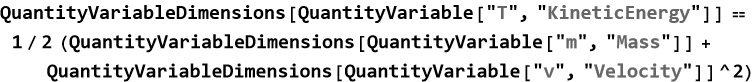
Exercise 13.17: Follow your textbook example symbolically.
Define QuantityVariables T (“KineticEnergy”), m (“Mass”), v (“Velocity”).
Compute QuantityVariableDimensions[T] and compare it (using ==) to the dimensions of m v² (i.e. QuantityVariableDimensions[m] + 2 QuantityVariableDimensions[v] — note the need to handle the exponent).
Use Thread or Map carefully to avoid the Thread::tdlen error you saw.
Conclude that T must be proportional to m v² (up to constant).Goal: Reproduce your logical proof entirely in WL.
Hint: Work with the list of rules returned by QuantityVariableDimensions, or use replacement rules like {“MassUnit” → M, “LengthUnit” → L, “TimeUnit” → T} for cleaner comparison.

Exercise 13.18: Define QuantityVariables: T (“Time” or “Period”), L (“Length”), g (“AccelerationDueToGravity”).
Use DimensionalCombinations[{T, L, g}, T] to find combinations that make T dimensionless.
Alternatively, compute IndependentUnitDimensions[{T, L, g}] (should be 2 independent dimensions).
Then use NondimensionalTransform[T / Sqrt[L/g]] and confirm it returns 1.
Explain how this shows T ∝ .Goal: Use WL to carry out the full pendulum derivation from your text.
Expected: One dimensionless combination: T or equivalent.

Exercise 13.19: Consider gravitational potential energy U near Earth’s surface.
Relevant variables: U (“Energy”), m (“Mass”), g (“AccelerationDueToGravity”), h (“Height” or “Length”).
a) Use DimensionalCombinations[{U, m, g, h}, U] to find the dimensionless group involving U.
b) Show via NondimensionalTransform that U/(m g h) is dimensionless.
c) (Advanced) Compare to kinetic energy: compute QuantityVariableDimensions[QuantityVariable[“U”,”PotentialEnergy”]] (if defined) or manually verify it matches m g h dimensions.
d) Discuss: Why can’t WL prove the coefficient is exactly 1 (unlike the 1/2 in KE)?

Power Output of a Machine

With some experience of dimensional analysis behind us, we turn to a fully detailed example. What determines the power output of a machine? We begin by listing every quantity that could possibly matter along with their dimensions.

Of course, the first quantity we are concerned with is the power output of the machine. Recall that we denote power with P. So what is power? It is the amount of energy per second. It has dimensions .

It seems reasonable to include the size of the machine. We will denote this as L with corresponding dimensions [L].

It also seems reasonable to consider the velocity of the moving parts of the machine, denoted v with dimensions .

Finally, we have the density of the material of the machine, denoted ρ with dimensions .

I am aware that this is a very simple view of a machine, but we are not considering a lot of other factors.

We now assume a power-law form in accord with the Rayleigh method.

(13.44)

where k is a dimensionless constant we do not yet know. So, (13.44) has dimensions

(13.45)

This gives us three equations for the various exponents. For mass [M],

(13.46)

For [L],

(13.47)

For [T],

(13.48)

Solving this system gives us, a=1, b=2, and c=2. This allows us to rewrite (13.44),

(13.49)

Order of Magnitude—Fermi Problems

“Give me five minutes and a pencil, and I’ll tell you the size of the universe—within a factor of ten.” Enrico Fermi

With exact numbers often unknown or unnecessary, we now learn the art of rough estimation. The technique that answers a question within a factor of 10 (sometimes 100) using only everyday knowledge is an order-of-magnitude estimate, also called a Fermi problem.

Enrico Fermi (1901–1954), the Italian physicist who created the first nuclear reactor and won the Nobel Prize in 1938, loved these questions. He would ask students:

“How many piano tuners are there in New York?” “How many grains of sand are on Earth’s beaches?” “How many molecules of air are in this room?”

Fermi showed that clever reasoning with big round numbers can get you astonishingly close.

The steps of a Fermi problem are:

Break the problem into smaller pieces you can guess.

Round every number to the nearest power of 10.

Multiply (or divide) the rounded numbers.

State the order of magnitude — “about ”.

Here are the classic Fermi problems.

Question                Fermi Estimate        Actual Value        Within factor
Piano tuners in New York (1950s)    ~150            ~190            ~1
Seconds in a year            3 ×             3.156 ×         ~1
Grains of sand on Earth’s beaches                        ~10
Mass of all humans            4 × kg        ~5 × kg        ~1

So, why bother with Fermi problems? First of all, beginning with an order of magnitude estimate gives you a constraint to compare detailed calculations with, if you are off by more than a factor of ten, you probably did something wrong and need to investigate what might have gone wrong. Secondly, as you do these you develop an intuition about the scales of the world. Third, it gives you a way to estimate what you don’t know.

Here are some detailed examples.

How many piano tuners are in New York City today?

We begin with the population of New York City ≈ people. Average household size ≈ 3 → ~3 × households. Fraction with pianos ≈ 1/20 → 1.5 × pianos. Pianos tuned once per year → tunings/year. One tuner can do ≈ 1000 tunings/year (4/day × 250 days). Therefore the approximate number of tuners ≈ 150 → order .

How many seconds are in a year?  60 s/min × 60 min/h × 24 h/day × 365 days ≈ 3 × s → order 10⁷ seconds.

How many molecules of air are in this classroom?  Room ≈ 10 m × 10 m × 3 m → volume ≈ 300 ≈ 3 × . 1 mole of air ≈ 22.4 L ≈ 2 × . Moles in room ≈ 3 × / 2 × ≈ moles. Avogadro’s number ≈ 6 × .  The number of molecules ≈ molecules.

How many grains of sand are on all the beaches of the world?  Average beach ≈ 100 m long × 30 m wide × 1 m deep → 3 × sand per beach. Number of beaches ≈ . Total sand volume ≈ . Grain of sand ≈ 1 = . Total grains of sand ≈ 3 × grains → order .

How much would sea level rise if all the ice on Earth melted?  Ice volume (Antarctica + Greenland) ≈ 3 × . Ocean surface area ≈ 3.6 × . Height increase ≈ 3 × / 3.6 × ≈ 80 m.

How many drops of water are in all the oceans?  Ocean volume ≈ 1.4 × L. One drop ≈ 0.05 mL = 5 × L. Drops ≈ 3 × drops.

Exercise 13.20: Estimate
a) How many heartbeats occur on Earth every second?
b) How many liters of blood are pumped by all human hearts in one day?
c) How many breaths do all humans take in one minute?
d) How many cups of coffee are drunk worldwide every day?
e) How many text messages are sent globally per second?
f) How many kilometers of road exist on Earth?
g) How much electricity does the entire human population use in one year?

Energy Used in Climbing Stairs

We now apply everything we have learned — units, dimensional homogeneity, order-of-magnitude reasoning — to a single everyday question: How much energy does a person use to climb one flight of stairs?

We solve it three ways: exact calculation, dimensional analysis, and pure Fermi estimation.

Given (rough numbers) that the mass of a person: m ≈ 70 kg. The height of one flight: h ≈ 3 m (≈ 15–20 steps). The acceleration due to to gravity: g ≈ 10 .

For the first approach to the problem, we will use some basic physics.

The minimum energy is just the gain in gravitational potential energy

(13.50)

(In reality, human efficiency is ≈ 20–25 %, so real energy used ≈ 8–10 kJ, since there are about 4 kJ per food calorie, so the stair climb would burn 2–3 food calories.).

The second method we use will be Rayleigh’s method.

We assume the energy depends only on mass, gravity, height,

(13.51)

with the dimensions

(13.52)

(13.53)

(13.54)

(13.55)

Solving the system gives us a=1, b=1, and c=1. Substituting these values into (13.51),

(13.56)

Dimensional analysis proves the formula must have this form — no other combination works.

The third method is the order of magnitude estimate (Fermi problem approach).

One flight of stairs is about the height of a small room, about m.

Gravity accelerates about 10 times harder than a gentle pull, about 10 .

Mass of a normal person is about 70 kg.

Using,

(13.57)

Exercise 13.21: Estimate
a) How many flights of stairs would you need to climb to offset a 1,000 food calorie lunch.
b) What is the energy expended by a push-up?
c) What is the energy expended by lifting a 10 kg weight above your head?
d) What is the energy expended by performing a pull-up?

Measuring Length

In order to measure distances and lengths, we must be able to locate a particle in a space. Given the fact that the point has no size or shape, and a particle is considered without regard to size or shape, we can say that a point is a mathematical structure that can describe the location of a particle.

This reduces our problem to finding a point representing the location of a particle within a space. The first thing to realize is that we cannot find the position of anything without knowing what that position is relative to. In other words, we have to identify some arbitrary reference point, for example where you are standing. We will call this reference point O. This is the classical notation for the origin. We can also set a point representing the location of the particle, called P.

We now recall Euclid's First Axiom: For every point O and every point P not equal to O there exists a unique line ℓ that passes through O and P. This line is denoted .

Any two points, O and P, and the collection of all points between them, that lie on the line , combine to form a line segment. Our segment is denoted .

The segment   is called the distance between O and P. We can measure this distance, denoted D(OP).

Recall that, given a number x the absolute value of x is x itself so long as x is greater than or equal to 0; if x is less than 0 then its absolute value is -x.

The Ruler Axiom states: Given a line ℓ, there exists a one-to-one correspondence between the points lying on the line ℓ and the set of real numbers such that the distance between any two points on ℓ is the absolute value of the difference between the numbers corresponding to the two end points. This is another way of stating that there is a distance interval. From this we can construct another expression for distance by applying the definition of the absolute value to the Ruler Axiom and then to the definition of distance we get,

(13.58)

To measure this we have to establish a unit of length. Let us say that this is a segment bounded by the points and .

We next have to find a point on such that ,

If we repeatedly apply something, we call it an iteration. We apply the unit length iteratively until we have n equal segments .

And thus the distance for the segment is then,

(13.59)

Thus, measuring distance is the iterative application of a unit of length n times and then adding any fractional remainders.

We can’t discuss a practical measurement without including the unit of measurement we are using. In this way the length of the segment becomes an algebraic quantity with the number of units being the coefficient of the symbol for the unit. We might say four feet, or ten point three six meters, or six and a half light years, etc.

Error in Measurement and Significant Figures

With length now defined as the iterative application of a unit plus any fractional remainder, we must face a hard truth: every real measurement is imperfect. No ruler is infinitely precise, no clock is perfectly stable, no human hand is perfectly steady. The difference between the true value that exists in nature and the number we write down is called error. The honest statement of how far our measurement might be from the truth is called uncertainty.

Errors come in two broad families. Systematic errors always push the result in the same direction: a ruler that has lost its first millimeter, a clock that runs slow, or reading a scale at an angle (parallax) will consistently make us overestimate or underestimate. Random errors scatter unpredictably around the true value: a slight tremor of the hand, a gust of wind, or tiny temperature changes cause readings to fluctuate from one trial to the next.

When we make a measurement it is vital to write it down correctly, the digits used are no more precise than what we can accurately measure—we call these digits the number of significant figures. There are some rules for significant figures:

All non-zero digits are significant. For example, 3.1416 has 5 significant figures.

Zeros between non-zero digits are significant. For example, 1007 has 4 significant figures.

Leading zeros are never significant. For example 0.0025 has 2 significant figures.

Trailing zeros are significant only when the number has decimal points. 2500 has 2 significant figures.

Exact number, whether counted or derived, have infinite significant figures.

The basic rule is that you must have the same significant figures  as the measurement having the fewest significant figures.

When we report a measurement, good practice demands that we state both the value and its uncertainty. We usually write 3.45 ± 0.03 m, meaning the true length very probably lies between 3.42 m and 3.48 m. The uncertainty is given to one or at most two significant digits, and the last digit of the central value is the first uncertain digit. This convention is the universal language of experimental physics.

A useful shorthand is the relative uncertainty, the absolute uncertainty divided by the measured value (often expressed as a percentage). A length of 3.45 ± 0.03 m has a relative uncertainty of about 0.9 %. When quantities are added or subtracted, we add the absolute uncertainties; when they are multiplied or divided, we add the relative uncertainties. These simple rules let us track how errors propagate through calculations.

In practice, the precision of an instrument limits how many digits we can trust. A typical meter ruler marked in millimeters allows us to estimate to about half a millimeter, so a reading of 1.237 m should be reported as 1.237 ± 0.002 m. Writing 1.237143 m would be dishonest; it suggests a precision we do not possess.

Wolfram Language makes uncertainty handling painless. We can write measurements as Quantity[1.237 ± 0.002, "Meters"] and let the software propagate the errors automatically. The result of a calculation appears with a realistic uncertainty, reminding us at every step that physics is an experimental science, not pure mathematics.

In the end, honest error analysis is what separates careful measurement from mere guesswork. A result without stated uncertainty is incomplete; a result with overstated precision is misleading. Learning to live with uncertainty—and to report it clearly—is one of the first marks of a real physicist.

Exercise 13.22: Estimate
a) Reading a Ruler. A student measures a table with a ruler marked in millimeters. She records 1243 mm.
    1) How should she properly report this measurement with realistic uncertainty?
    2) Convert to meters and report with correct significant figures.
b) Adding Measurements. Measured lengths are: 12.51 cm, 3.2 cm, 0.134 m.
    1) Add them and report the sum with correct uncertainty/decimal places.
    2) Explain why your answer has the precision it does.
c) Multiplying with Different Precisions. A brick has mass 2.45 ± 0.05 kg and volume 0.900 ± 0.015 L. Calculate density (kg/L) and give the result with proper significant figures and uncertainty.
d) Propagation of Percentage Uncertainty. Speed is calculated as where distance = 250.0 ± 0.5 m, time = 12.34 ± 0.06 s.
    1) Calculate percentage uncertainties in d and t.
    2) Find percentage uncertainty in v.
    3) Give final answer for v with correct significant figures.
e) Real Laboratory Data. A student records these repeated measurements of the same length (cm): 8.42, 8.39, 8.44, 8.41, 8.40.
    1) Calculate the average and the estimated uncertainty (use ± half the range as a rough estimate).
    2) Report the final result properly.
f) Significant Figures Trap. A calculator gives: 1.234+5.6789×0.02=1.347778. Explain step-by-step why the correct answer is 1.3 (not 1.347778) and state the rule that forces this.

Data Analysis

With measurements now accompanied by uncertainty, we turn to the art of extracting meaning from numbers. The process of finding the underlying pattern in experimental data is data analysis.

The goal that guides us is to discover a simple mathematical relationship that describes the data well enough to predict new values is what we call an empirical formula.

We take a table of measured points and ask the question, “What is the simplest equation that passes close to all these points?”

Common choices (in order of increasing complexity):

Linear          y = a + b x  

Quadratic      

Cubic            

Quartic        

The method that finds the coefficients a, b, c, … that minimize the total squared error is least-squares fitting. We will delve deeply into this method later.

For now, we can use WL to this for us. We use the Fit command.

For now we will only consider the first definition.

Let’s say that we have a collection of data.

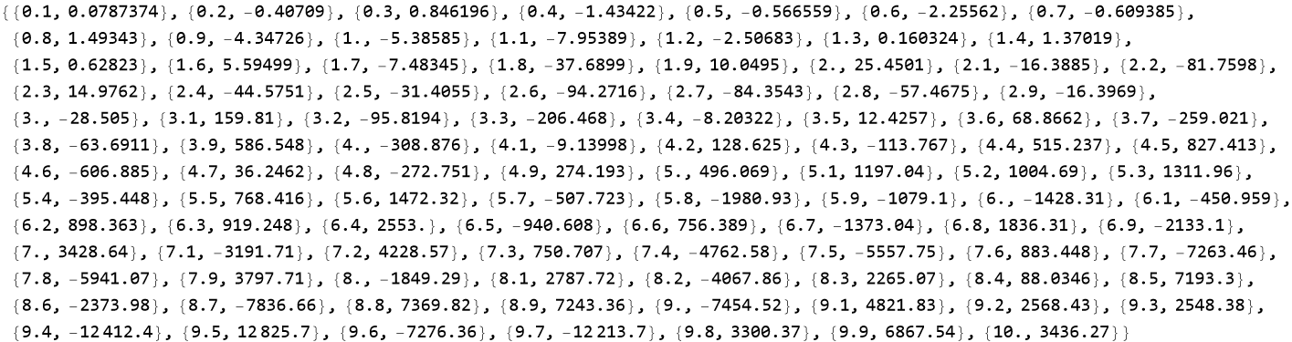
We can see a plot of this collection.

To find the expression for fitting, we start with a straight line.

We can plot this along with the data.

As you can see, this fits well until about 4 and then it stops doing so well. Let’s try fitting a quadratic.

with

so

This seems little better. We now try a cubic fit.

with

so

This is beginning to look better, but it is not good enough. We move up to quartic.

with

so

Even better, so it seems if we go to higher degree polynomials that we might be able to fit this.

When you find a good fit, then you have a formula, this formula will fit your data, so it is an empirical formula for your data.

Exercise 13.23: Generate a small dataset of 15 points where y ≈ 3.2 x + 7, but with moderate random noise (±4 units).
a) Use Table + RandomReal to create the data:
   data = Table[{x, 3.2 x + 7 + RandomReal[{-4,4}]}, {x, 0, 14, 1}];
b) Plot the points with ListPlot[data].
c) Fit a straight line using Fit[data, {1, x}, x].
d) Plot the fit together with the data using Show[ListPlot[data], Plot[fit, {x,0,14}]].Goal: See how well a linear model captures noisy but basically linear behavior.
Expected insight: The fit coefficients will be close to {7, 3.2}, but not exact — noise matters.

Exercise 13.24: Create data that is truly quadratic: . Use x from 0 to 8 in steps of 0.5 (17 points).
a) Plot the raw data.
b) Fit both a line ({1,x}) and a quadratic ({1,x,x²}).
c) Use Show to overlay both fits on the data points (different colors).
d) Visually judge: which fit looks better? Compute the approximate maximum deviation for each.Goal: Experience the danger of under-fitting (linear model misses the curvature).
Expected insight: Linear fit looks systematically wrong (residuals form a parabola); quadratic hugs the points much better.

Exercise 13.25: Use the same quadratic data from Exercise 2.
a) Fit polynomials of degree 1, 2, 4, 6, and 8.
   Example: Fit[data, Table[x^i, {i,0,deg}], x]
b) Plot all five fits on the same graph with the data points (use different colors or styles).
c) Extend the plot range to x = −2 to 10 (beyond the data).  Goal: See what happens when you use too high a degree.
Expected insight: Low degrees underfit, degree 2 fits well, higher degrees oscillate wildly outside the data range (classic overfitting).

Exercise 13.26: Generate pendulum-like data: period .
Use L from 0.2 m to 2.0 m in steps of 0.2 m (10 points), g ≈ 9.8 m/s², add ±0.05 s noise.
a) Create dataT = Table[{L, 2 Pi Sqrt[L/9.8] + RandomReal[{-0.05,0.05}]}, {L,0.2,2.0,0.2}];
b) Since ∝ L, fit vs. L to a line through origin: /. }, {L}, L].
c) Extract the slope → estimate g = 4π² / slope.
d) Compare to direct nonlinear fit if curious: NonlinearModelFit[dataT, a Sqrt[L], a, L].Goal: Connect data fitting to physical laws (dimensional thinking → empirical confirmation).
Expected insight: Slope ≈ 4π² / 9.8 ≈ 4.03–4.05; recovered g close to 9.8.

Exercise 13.27: Take your original noisy data from the chapter notebook (the one that went up to degree 4).
a) Compute fits of degree 1 through 5.
b) For each fit, calculate the sum of squared residuals:
   Total[(y - fit /. x -> #[[1]])^2 & /@ data]
c) Make a table: degree vs. sum of squared errors (SSE).
d) Plot residuals (y − predicted) vs. x for degree 2 and degree 5.Goal: Introduce quantitative comparison (beyond eye-balling).
Expected insight: SSE drops dramatically from linear → quadratic → cubic, then decreases only marginally (or even increases slightly due to noise fitting) → diminishing returns + risk of overfitting.

Experiment Design

With measurement, units, error analysis, and data fitting now in hand, we can finally answer the most important question of experimental physics, “How do we design an experiment that actually tells us something true about nature?”

Good experiment design is nothing more than the deliberate application of everything we have learned in this chapter.

The Core Principles of Experiment Design:

Ask a clear, testable question.

“How does period depend on length?” is good.

“What affects a pendulum?” is too vague.

Choose the right variables

Independent variable – the quantity you deliberately change (length L).  

Dependent variable – the quantity you measure (period T).  

Controlled variables – everything else you keep constant (mass, angle, air pressure).

Use dimensional reasoning first

Before touching equipment, ask: “What must the answer look like?”

For the pendulum: T must be ∝ — this tells us we only need to vary L and measure T.

Plan the range and spacing

Cover at least one order of magnitude (e.g., L from 0.1 m to 2 m).  

Take 6–10 data points — enough for a clear trend, few enough to finish in one lab session.

Estimate uncertainty before you start

Ruler precision ≈ ±1 mm → Δ L/L ≈ 1 % at L = 10 cm, 0.1 % at L = 1 m.

Choose lengths where uncertainty in T is measurable but not overwhelming.

Repeat measurements

Three trials at each length reduces random error by roughly .

Record everything in proper units and significant figures

Example entry:
L = 0.750 ± 0.001 m,   T = 1.74 ± 0.02 s (average of three swings)

Fit the data and check the theory

Plot versus L → should be a straight line through origin with slope = 4π²/g.

Use Fit[data, {1, x}, x] → extract g and its uncertainty.

State the final result with honest uncertainty

“g = 9.81 ± 0.07 m/s² (0.7 % uncertainty)”

Here is a real checklist you can use tomorrow:

Clear question?  

Variables identified and controlled?  

Dimensional analysis done?  

Range covers order of magnitude?  

Uncertainty estimated?  

Enough repeats?  

Units and significant figures correct?  

Fit matches theory?

In science, a well-designed experiment is one where nature is given no choice but to reveal her secrets. Master these steps, and you are no longer just collecting numbers — you are doing real science.

Scaling Laws

With dimensional analysis, order-of-magnitude estimation, and the Rayleigh Method now in hand, we can answer one of the deepest questions in physics without doing a single experiment, “How does a physical quantity change when we make the entire system bigger or smaller?” The relationships that tell us exactly that are called scaling laws.

A scaling law is nothing more than the result of dimensional analysis applied to size.

We simply ask: “If every length in the system is multiplied by a factor λ (lambda), how does every other quantity change?”

The Master Formula

If a quantity Q has dimensions

(13.60)

then when all lengths are scaled by λ such that Q   →   Q λ a (mass scaling)b (time scaling)c …
Classic Scaling Laws (derived in 30 seconds each)

System                What we scale        Resulting scaling law                        Real-world consequence
Strength of a bone        Length λ        Force ∝ area ∝                         Elephants need thick legs
Metabolic rate of animals    Length λ (mass ∝ )    Power ∝ ≈                         Mice need to eat more per gram than elephants
Speed of a sailing ship        Length λ        Max speed ∝ ∝ (wave drag)                Bigger ship = faster
Flight speed of birds/insects    Length λ        Speed ∝                             Dragonflies can’t be bus-sized
Period of a pendulum        Length λ        T ∝                             A 100-times longer pendulum swings 10 times slower
Energy to crush an egg        Length λ        Energy ∝ (volume) but strength ∝ → fails at large size    Why dinosaurs needed thick eggs
Everything in biology, engineering, and astrophysics is governed by these scaling exponents that dimensional analysis reveals before any experiment. In physics, scaling laws are the hidden reason why “big” and “small” are completely different worlds.

Summary

Write a summery of this chapter.

For Further Study

L. A. Sena, (1972). Units of Physical Quantities and Their Dimensions, Mir Publishers. A very good book that covers all topics of this lesson and a lot more.

D. C. Ipsen, (1960), Units, Dimensions, and Dimensionless Numbers. McGraw-Hill Book Company, Inc. This is my favorite book by one of the people who developed the field.

Dimensional Analysis and Scaling, 3Blue1Brown, https://www.youtube.com/watch?v=0X7mA7J6qI4

Error Analysis and Significant Figures, Eddie Woo, https://www.youtube.com/watch?v=2Yq4b7l6Q2s

Fermi Estimation and Order of Magnitude, , The Math Sorcerer, https://www.youtube.com/watch?v=1X4wK5pB3fM

Dimensional Analysis in Physics, Michel van Biezen, https://www.youtube.com/watch?v=3gq9pT8H2E4