Classical Mechanics
George E. Hrabovsky
MAST
Introduction
Before delving into the marvels of quantum mechanics, it is a good idea to review some important ideas from classical mechanics. I assume that Newtonian mechanics is not a mystery.
Generalized Coordinates
One of the basic problems in classical mechanics is to predict where a particle will be at some given time. To do this we choose to represent the space the particle is in by a coordinate system. When we consider coordinates that allow us to specify the location of a particle, then we have a generalized coordinate system, or just generalized coordinates. Such coordinates are often labeled by ![]() for m-dimensional space.
for m-dimensional space.
For a single particle in 3-space, there are 3 q's (corresponding to the Cartesian axes x,y,z). For any system having two particles there are 6 q's (corresponding to the x,y,z for each particle). For a system with ![]() particles, there are
particles, there are ![]() q's.
q's.
We know the q's are not enough to predict the future of the system; you must also know the velocities, ![]() 's, these are called the generalized velocities.
's, these are called the generalized velocities.
Usually you need 6 n pieces of information to be able to predict the future of n particles.
CM-1: Why are there 6 n pieces of information?
What does it mean to predict the future? It means to specify a set of functions, ![]() ,
, ![]() , ...,
, ..., ![]() . These functions are the generalized coordinates in m-space of n particles in time. This set is called the generalized trajectory of the system. We can represent this situation by a diagram. We will use the representation of a horizontal plane for all of our q's, even though the picture is only two dimensional (see Figure CM-1).
. These functions are the generalized coordinates in m-space of n particles in time. This set is called the generalized trajectory of the system. We can represent this situation by a diagram. We will use the representation of a horizontal plane for all of our q's, even though the picture is only two dimensional (see Figure CM-1).
Figure CM-1: The generalized coordinates.
Vertically we will plot the time (see Figure CM-2).
Figure CM-2: Generalized coordinates and time.
A trajectory is a value for the q's at every time (see Figure CM-3).
Figure CM-3: A generalized trajectory.
We might not really be interested in every single trajectory, were we to have a system with ![]() particles then determining the trajectory of the system is equivalent to determining the trajectories of all
particles then determining the trajectory of the system is equivalent to determining the trajectories of all ![]() particles. Nobody tries to do that, in such a system we would make statistical statements or some approximation (for example, we might consider the system to be a continuum, like a fluid). That said, the central problem of classical mechanics is to determine the trajectory of a particle.
particles. Nobody tries to do that, in such a system we would make statistical statements or some approximation (for example, we might consider the system to be a continuum, like a fluid). That said, the central problem of classical mechanics is to determine the trajectory of a particle.
Using Newton's equations of motion, given the q's and the ![]() 's, we can determine the trajectory
's, we can determine the trajectory ![]() . If we zoom in on the trajectory so that we see it as a collection of points, Newton's equations of motion tell us how to move from one point to the next (see Figure CM-6).
. If we zoom in on the trajectory so that we see it as a collection of points, Newton's equations of motion tell us how to move from one point to the next (see Figure CM-6).
Figure CM-6: Zooming in on the generalized trajectory.
This is a good law of dynamics, since there is one arrow into each state and one arrow out of it.
Newton's equations of motion are ordinary differential equations. Since we do not need to know the entire trajectory we call them local; a standard quality of differential equations. All we need to know is where we are right now and how we will move in the next instant. If you know all of these points, then you can build up the entire trajectory small piece at a time—this is called an initial-value problem.
The Principle of Stationary Action
We now begin another formulation of classical mechanics, one that looks at the trajectory as a whole. Instead of being given the position and velocity at a single time, you are given the position at the beginning of the trajectory and, after a certain passage of time, the position at the end of the trajectory. We have a particle with the starting point ![]() and the end point
and the end point ![]() . There is only one trajectory connecting those two points (see Figure CM-7).
. There is only one trajectory connecting those two points (see Figure CM-7).
Figure CM-7: The unique trajectory connecting the end-points.
If the object leaves ![]() with the wrong velocity, it will never reach
with the wrong velocity, it will never reach ![]() . We have the same number of things we need to know as before; instead of the position and velocity we have the position at two specific times.
. We have the same number of things we need to know as before; instead of the position and velocity we have the position at two specific times.
The guiding principle is that there is some quantity, the action, based on the entire trajectory that is a local minimum. This is called the principle of stationary action. It is sometimes called the principle of least action. In this regard we know we are on the correct trajectory as any deviation will cause an increase in the action.
Let's take our two points and calculate the length of the curve connecting them. The curve that minimizes this length is a straight line (see Figure CM-8).
Figure CM-8: The shortest curve.
The action is not a function of a finite number of variables; it is a function of every point along the trajectory. This is a much more complicated object than minimizing a function of a few variables. There are two approaches to this problem.
The first approach is what we examined above; you pick your two points, take the length of the trajectory, and then you ask what curve minimizes that length? This is called the global approach since it takes into account the entire trajectory.
The second approach requires us to break the trajectory into distances between points. If we zoom in on these points we see something like Figure CM-9
Figure CM-9: Zooming in on the trajectory.
In the case of every local interval we have a starting point and an ending point. This approach does not depend on the entire trajectory, you only need to know the two local end-points of the interval you are considering. This is called the local approach; if you know these two local points, then the rest of the trajectory doesn’t matter. The midpoint is placed so that the particle proceeds straight ahead. We could write this as a differential equation stating that the slope from one point to the next in the length is zero. If we know the location of each point, and we tell the particle to go straight ahead from each point, then the shortest distance will be a straight line.
We can call these two ideas the global and local versions of the principle of least distance.
The Mathematical Formulation of the Principle of Least Action
We define two points, ![]() and
and ![]() (see Figure CM-10).
(see Figure CM-10).
Figure CM-10: Two points on the x-y plane.
These will be our endpoints. We also have a curve between them (see Figure CM-11).
Figure CM-11: The curve between the end-points.
The first thing we need to do is calculate the length of a curve and then minimize it. We then take a thin slice, whose thickness is dx along the x axis (see Figure CM-12).
Figure CM-12: Taking a thin slice of width dx.
We can zoom in on this interval (see Figure CM-13).
Figure CM-13: Zooming in on the interval.
We can also indicate dy (see Figure CM-14).
Figure CM-14: The intervals dx and dy.
As we go from x to x+dx, the function goes from y to y + dy. The length of the curve here can be approximated as the length of the hypotenuse of a right triangle. If we add up all of the lengths of the hypotenuses then we will have the overall length of the curve.
Traditionally, any distance along a curve is denoted s, not to be confused with speed. The differential of this curve length is called the line element and is written, ds. In our situation (Figure CM-14) we can say that the square of the line element is,
![]()
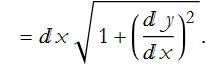
then the line element is,
![]()
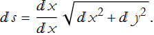
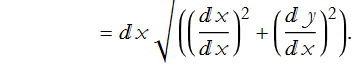
We can manipulate the radical by multiplying through by dx/dx,
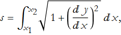
Now we add up the distances of all of the line elements to find the total length of the trajectory. Since we have an infinite number of points in any interval, we must take an integral. Thus, the total distance from ![]() to
to ![]() is,
is,
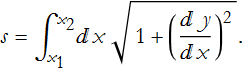
So our problem is to find the function y(x) that makes s a minimum. We must make  larger than one. If you add 1 to something positive the sum is also positive, then the
  term must be positive. If the derivative was 0 there would be no change iny with respect to x and it would be flat and the curve would not go between the two points.
Given that the curve must go between the two points we must make the integral as small as possible Now, we don't yet know how to calculate this, we have simply formulated the problem mathematically.
The s in Eq. (CM.1) can be thought of as a function of y, itself a function; a function of a function. Given y(x) we have a rule for calculating a number, s, from it. There is a name for a number that depends upon the totality of a function, we call it a functional. So, a functional is the function of a function. The output is a number, while the input is a function.
We then state that the distance between two points is a function of y, and thus it is a functional. Our task is then to minimize this functional, subject to the condition that the curve passes through two specific points.
The Calculus of Variations
Here is a famous situation where you might want to minimize a quantity with respect to an entire function; determining the shape of a weighted string or cable, of a given length, hung between two points (see Figure CM-15).
Figure CM-15: A string hung between two points.
It is a curve that always minimizes the potential energy. Potential energy is a function of height, where getting higher means a higher potential energy; minimizing it means the string or cable gets as low as it possibly can. It can't go through the ground beneath it, because it has a fixed length. What if we go straight down, then across and up again (see Figure CM-16)?
Figure CM-16: An alternate configuration.
This is not the most efficient configuration either. In the center we could do a better job of minimizing the potential energy (see Figure CM-17).
Figure CM-17: The problem.
The curve that describes this condition is a catenary. We will not go any deeper into this curve’s behavior. This is an example of where you want to minimize some quantity with respect to a function, in this case a curve.
The mathematics that describes how you minimize a functional with respect to a function is called the calculus of variations. The principle of least distance is of this character; we are minimizing some functional with respect to the whole trajectory. Here we are not talking about just one function, but we have ![]() that produce the entire trajectory (see Figure CM-18).
that produce the entire trajectory (see Figure CM-18).
Figure CM-18: The generalized trajectory.
The principle of stationary action tells us that there is some action, such that when we minimize it with respect to the trajectory it is equivalent to Newton's laws of motion.
Which formulation is more efficient, or more easy to use, depends on the problem at hand. It would take a long time to write out all the forces between all of the components of a normal object—with its ![]() particles and
particles and ![]() coordinates. On the other hand, if we know how this normal object is moving between two points with a given action, and that the trajectory minimizes that action, the problem becomes much easier.
coordinates. On the other hand, if we know how this normal object is moving between two points with a given action, and that the trajectory minimizes that action, the problem becomes much easier.
It is important to realize that where Newton's laws apply, the two methods are equivalent. This is the most general formulation of the laws of classical mechanics; though you might have to generalize the principle for situations where you have fields or waves.
The Action
The form of the action, S, is a bit surprising. We will have to prove that it produces the same results as Newtonian dynamics. Once we have done that, then we will have a reason to believe it.
We need to calculate the kinetic energy T and the potential energy V, and then integrate with respect to time. Assume that we have one particle in one dimension. The problem will be to find the trajectory, in this case x(t) such that the action is minimized. Since this is about energy, you would expect us to write something like this, for the action.
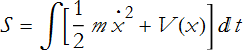
It seems reasonable to say that for each instant of time the action would be the sum of the total energy and the time interval. This is wrong! Eq. (CM.2) is almost correct, in reality the action is defined,
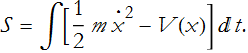
The action is really the time integral of the kinetic energy minus the potential energy! This formulation comes about because the force is the negative gradient of the potential energy.
We can compare this with the principle of least distance. From the principle of least distance we have,
This case depends on the function and its derivative with respect to the independent variable. The action also depends on the function, V(x(t)) as a function of time and the time derivative, ![]() . In both cases we now have a dependence on the function and its derivative with respect to the independent variable. All are integrals along the independent variable. In both cases we also have two fixed points and we are trying to minimize the functional (distance or action) along the curve joining the points (see Figure CM-18).
. In both cases we now have a dependence on the function and its derivative with respect to the independent variable. All are integrals along the independent variable. In both cases we also have two fixed points and we are trying to minimize the functional (distance or action) along the curve joining the points (see Figure CM-18).
Figure CM-18: The variational principles.
These are called variational principles. It is important to realize that fixed points do not vary in the coordinate system. In the case of least distance they are in spatial coordinates, in the case of stationary action they are in space as a function of time.
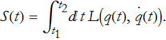
The integrand in Eq. (CM.3) can be rewritten for generalized coordinates,
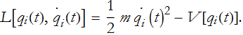
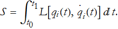
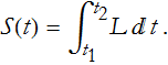
This is called the Lagrangian and is symbolized by L. The action is then the integral over time of the Lagrangian from the beginning, ![]() , to the end,
, to the end, ![]() , of the trajectory. So, the most general version of the action is,
, of the trajectory. So, the most general version of the action is,
The most general statement of the principle of stationary action is that for any mechanical system you have the Lagrangian, out of which you build the action, then you find the path that minimizes that action. In all cases where this corresponds to Newton's laws the Lagrangian is the difference of the kinetic energy and the potential energy. In systems that have no Newtonian analog this Lagrangian may look completely different, but it will still depend on the generalized coordinates and velocities. The principle of stationary action is more fundamental than any Newtonian principle of mechanics.
7.2 Integration by Parts
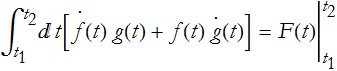
Suppose that we have the product rule for the derivative of a product F(t)=f(t) g(t)
![]()
How do we integrate this? We can write
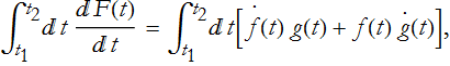
or,
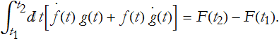
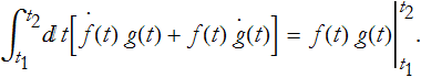
The standard notation for the right hand side is,
![]()
We can now write the integral,
since F(t)=f(t)g(t),
Let's take the special case where either f or g vanishes at the end points. Different cases of this could be f becoming 0 at the two end points, g becoming 0 at the end points, or a mixed case. In this case we can rewrite the integral,
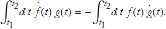
When we have the product of a derivative and a non-derivative in the integrand, we can switch which function is differentiated by changing the sign of the integral. This is only true if the definite integral of the product is 0.
7.5 Lagrange’s Equations
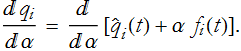
We are going to derive a differential equation (a local law) from a global law. Let's start by saying that the trajectory, the solution to the problem, is given by ![]() , where N is the total number of coordinates required to describe the system. We can change the trajectory by transforming the coordinates according to the rule,
, where N is the total number of coordinates required to describe the system. We can change the trajectory by transforming the coordinates according to the rule,
![]()
where α is some coefficient of the arbitrary set of functions ![]() . We also require that the new trajectory pass through the same end points. Another way of stating this condition is that
. We also require that the new trajectory pass through the same end points. Another way of stating this condition is that ![]() for the end points
for the end points ![]() and
and ![]() . Figure CM-19 shows us the shifted trajectory.
. Figure CM-19 shows us the shifted trajectory.
Figure CM-19: The shift in trajectories.
At each point t, other than ![]() and
and ![]() , the trajectory
, the trajectory ![]() is shifted in a manner proportional to
is shifted in a manner proportional to ![]() , and these functions are themselves shifted by α. This trajectory is not a solution of the equations of motion.
, and these functions are themselves shifted by α. This trajectory is not a solution of the equations of motion.
It is important to note that if we shift the trajectory, then the action becomes a function of α, S(α), since the new trajectory depends on the amount that you shifted the trajectory.
Let's say that we know that the action is minimized for the true trajectory. This corresponds to the situation when α=0. The principle of stationary action tells us that S(α) is minimized for every possible collection of functions ![]() ,
,
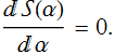
for every ![]() when α=0. Any change in the parameter α increases the action. In other words S(α) is stationary when α=0.
when α=0. Any change in the parameter α increases the action. In other words S(α) is stationary when α=0.
The action must be connected in some way to Newton's equations. The action is the integral of a thing, called the Lagrangian, from ![]() to
to ![]() along the trajectory,
along the trajectory,
The Lagrangian is named for Joseph-Louis Lagrange, an Italian-born physicist and mathematician.
The action is the integral, the sum of all of the tiny bits of the Lagrangian, along the whole trajectory. The whole trajectory is the sum of a lot of little pieces. Each piece will have its own action. The total action for the trajectory is the sum, or integral, of these tiny actions.
The trajectory is being varied by a small shift (see Figure CM-20). The trajectory that we want is the one having the least action,
We can see that S is a function of α because the q's are functions of α. Let's write,
![]()
where the carat symbol ^ represents the true solution to the problem of finding the correct trajectory (see Figure CM-20).

Figure CM-20: The true trajectory ![]() and the shifted trajectory
and the shifted trajectory ![]() .
.
We can see then that ![]() is a function of α for any t. What is the derivative of
is a function of α for any t. What is the derivative of ![]() with respect to α?
with respect to α?
We know that ![]() is not a function of α, so its derivative with respect to α is 0. This leaves,
is not a function of α, so its derivative with respect to α is 0. This leaves,
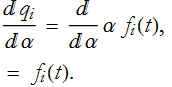
So the change in ![]() with respect to α is just
with respect to α is just ![]() . What about the change in the velocity? How does the velocity change when you change α a little bit?
. What about the change in the velocity? How does the velocity change when you change α a little bit?

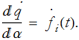
We can write,
![]()
So its derivative with respect to α is going to work the same way that we got Eq. (CM.11) from Eq. (CM.10). The answer will be,
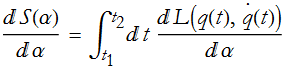
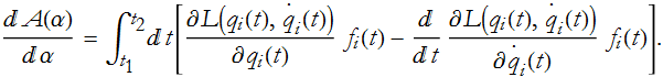
How much does the action change when you vary α by a little bit? We differentiate S with respect to α.
The Lagrangian is a function of two variables. We have the total derivative of the Lagrangian. For a general function of more than one variable, B(x(t),y(t)), the total derivative is
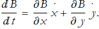
Applying this, we can rewrite Eq. (CM.13),
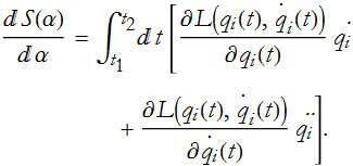
Using Eq.s (CM.10) and (CM.11) we can change this to,
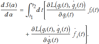
Another way of saying this is that the change in a function is the change in the function with respect to each argument times the change in that argument, summed over all arguments. We use the word argument in this sense to mean independent variables. So we differentiated by each of the variables within L, and multiplied by the change of that variable. Now, here we have a term with ![]() in it, recall that this can be any function at all—with one restriction, it vanishes at the end points.
in it, recall that this can be any function at all—with one restriction, it vanishes at the end points.
Here we have ![]() , it would be nice to have
, it would be nice to have ![]() there instead; then we would have a sum multiplied by an arbitrary function.
there instead; then we would have a sum multiplied by an arbitrary function.

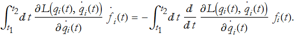
What's the trick to turn this into ![]() ? Integration by parts!
? Integration by parts!
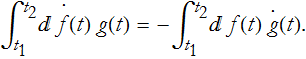
In our case we are going to "undifferentiate" ![]() by changing signs and differentiating
by changing signs and differentiating 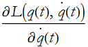 . Specifically,
or
we can take the ![]() 's out of the brackets,
's out of the brackets,
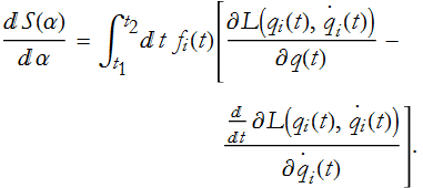
We can see the structure of the relationship, we have this term because we are changing q a little bit,
We have this term because we vary ![]() a little bit.
a little bit.
Now what about the end points? Recall the term ![]() . Since we stipulated that
. Since we stipulated that ![]() was zero at the end points, this term vanishes and plays no role. So Eq. (CM.16) is the change in action with respect to α. We already know that this must be 0, as a consequence of minimizing the action,
was zero at the end points, this term vanishes and plays no role. So Eq. (CM.16) is the change in action with respect to α. We already know that this must be 0, as a consequence of minimizing the action,
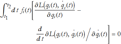
and this must be true for every possible ![]() since we are looking for the minimum possible action, no matter what function we use to deform it. Any deformation in the trajectory will add a little action. It follows from this that the integral must always be 0. This implies that the quantity in the bracket must be identically equal to 0,
since we are looking for the minimum possible action, no matter what function we use to deform it. Any deformation in the trajectory will add a little action. It follows from this that the integral must always be 0. This implies that the quantity in the bracket must be identically equal to 0,
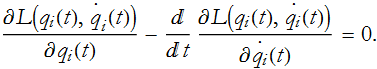
So, what we have done is taken a global statement of the principle of least action and converted it into a local statement at each point along the trajectory. This is true for every combination of ![]() 's for all times and points. Equation (CM.17) is a local equation that is equivalent to the global statement that the action is a minimum and is called the Euler-Lagrange Equation, (pronounced oiler-Lagrange), or just the Lagrange equation, for the variational problem of finding the trajectory that minimizes the action. This equation, in one form or another, is the heart of all of physics! Any problem of a physical system can be formulated as an action principle with a Lagrangian.
's for all times and points. Equation (CM.17) is a local equation that is equivalent to the global statement that the action is a minimum and is called the Euler-Lagrange Equation, (pronounced oiler-Lagrange), or just the Lagrange equation, for the variational problem of finding the trajectory that minimizes the action. This equation, in one form or another, is the heart of all of physics! Any problem of a physical system can be formulated as an action principle with a Lagrangian.
We will see that Eq. (CM.17) produces the correct equations of motion. At a fundamental level, this is the relationship between a global statement of the principle of least action and a system of differential equations that we will find have the basic form F=m a.
Now we are going to introduce some definitions. We begin with,
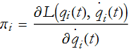
this is called the momentum canonically conjugate to q. Here you think of the ![]() 's as positions, then the
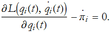
's as positions, then the ![]() 's are the momenta. So, substituting Eq. (CM.18) into Eq. (CM.17) we have,
's are the momenta. So, substituting Eq. (CM.18) into Eq. (CM.17) we have,
This tells us that the time derivative of the momentum is equal to the partial derivative of the Lagrangian with respect to position,
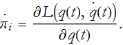
Since the left-hand side of Eq. (CM.19) has a name, does the right hand side? Yes, it is the generalized force. The derivative of the momentum is the force, and we have Newton’s second law of motion.
Click here to go back to the quantum mechanics page.
Click here to go back to our home page.