The Dirac Delta and Green's Functions
George E. Hrabovsky
MAST
Introduction
We all know about particles. Classically they occupy a point, and the mathematics has been built-up around that concept. There is often a need to consider a density (mass, energy, charge, etc.) for objects being represented as particles. How do we get around the fact that the volume of a particle is zero?
The Idea of a Dirac Delta—A First Approach
How can we develop a mathematical object that has a radius within an arbitrarily close distance of zero? In fact we must force this distance to be indistinguishable from zero—what we call a neighborhood around zero. We must also make sure that this region has some area to it that is more than 0 (positive). Why? There is no point in considering such an object otherwise—the goal is to make something where any density will not become infinite, so its area/volume has to be larger than 0. We are effectively asking to be able to make a concentration of the essence of an object into a very small, but non-zero, region. We can make this a definition of our mathematical object: A positive area concentrated into the neighborhood of zero. The density of this region, its integral, will be 1. This is what we call the Dirac Delta. Some have said of it, “It is higher than the Devil and narrow as Hell.” We will denote this object with the symbol δ(x). Were we to plot this, it would look like this,
Figure DDG-1: The Dirac Delta.
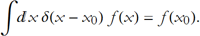
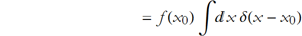
Some careful consideration, which we do not have time for right now, will lead to the following property, for any non-pathological univariate function f(x),
DDG-1: Why is this true?
Since we are in the neighborhood of ![]() we can specify this neighborhood by establishing the interval
we can specify this neighborhood by establishing the interval ![]() , for a sufficiently small ε. Since our function is not pathological, it will not blow up at
, for a sufficiently small ε. Since our function is not pathological, it will not blow up at ![]() . By our definition f(x) will not vary anywhere within the neighborhood. Thus
. By our definition f(x) will not vary anywhere within the neighborhood. Thus ![]() in the neighborhood. We can then write
in the neighborhood. We can then write

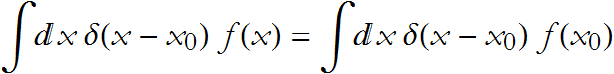
Since ![]() does not change over the interval, it is a constant. so,
does not change over the interval, it is a constant. so,
From our original specification,
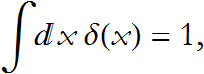
so

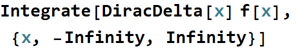
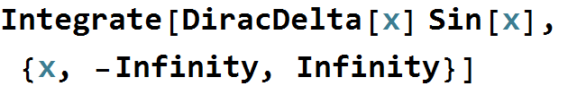
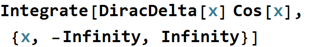
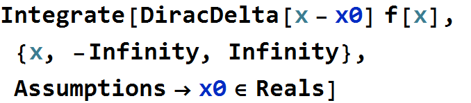
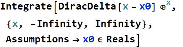
We can see some examples of this.
![]()
![]()
![]()
![]()
![]()
Many problems lead to a Dirac delta.
Properties of the Delta
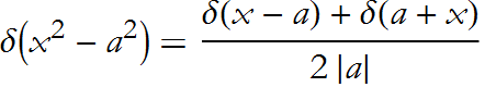
The first property is that the Dirac delta doesn’t care about sign.
![]()
![]()
Other properties are:
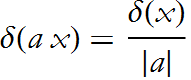
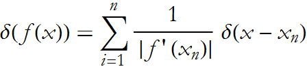
here ![]() are the roots of f(x).
are the roots of f(x).
If have an integral of the form,
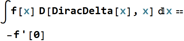
we see that this is the equivalent of a difference from the product of the Dirac delta and the initial value of our function, and the product of a new function by the derivative around the initial value of the function. But what the heck is represented in Mathematica by the HeavisideTheta? In normal mathematics we call this the step function.
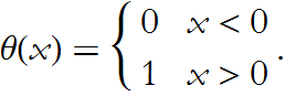
The Step Function
The step function is defined as follows,
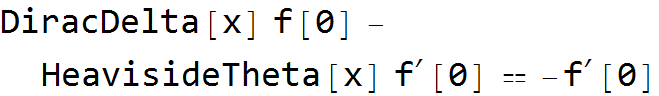
Thus the integral above becomes
![]()
The derivative of an arbitrary step function is the Dirac delta.

![]()
From this we see another way to define the step function, as the integral of a Dirac delta.
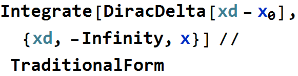
![]()
Green’s Functions
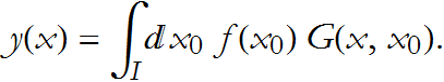
Let’s say we have the differential equation
![]()
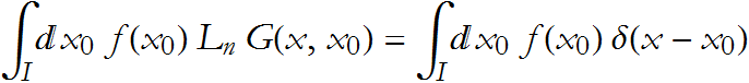
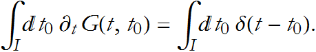
We can think of f(x) as the input and ![]() as the output. What happens when the input is a Dirac delta? This converts the differential equation into the form
as the output. What happens when the input is a Dirac delta? This converts the differential equation into the form
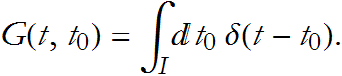
![]()
over some interval ![]() . If we know what G is, then we have solved the differential equation.
. If we know what G is, then we have solved the differential equation.
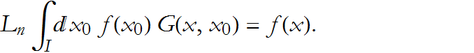
If we compare this with (DDG.6), we can see that
So, G is what we call a Green’s function, named for the British mathematician George Green (1793 - 1841).
This example is due to Hermann Schultz’s book, “A Theoretical Physics Primer,” 2015, published by Verlag Europa-Lerhmittel. We will examine the falling body problem, where we have one-dimensional motion a(t)=-g. Thinking about it, we need our interval I to be a time interval, (0,T), with T being some later time. The operator is ![]() . We can then write the characteristic equation
. We can then write the characteristic equation
![]()
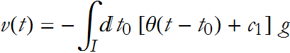
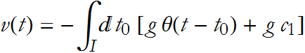
Integrating this, we have
![]()
This gives us an expression for the velocity
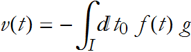
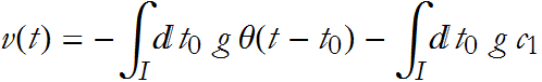
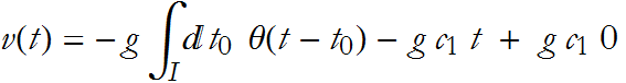
If, as ![]() we have the condition
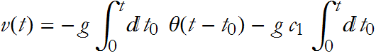
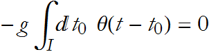
we have the condition ![]() then we say that the operator exhibits translational invariance. In this case the left hand term vanishes,
then we say that the operator exhibits translational invariance. In this case the left hand term vanishes,
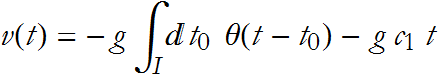
we then have a familiar looking solution,
![]()
where the constant ![]() is the only thing unfamiliar.
is the only thing unfamiliar.
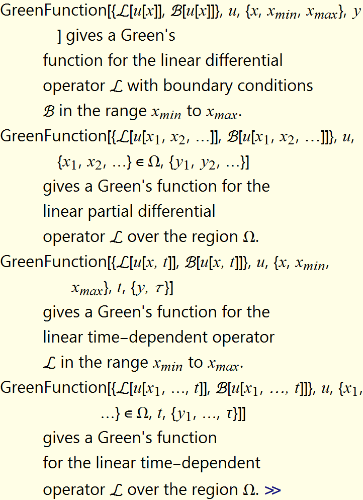
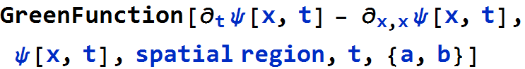
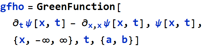
Mathematica allows you to work with Green’s functions.
![]()
So let’s try this for the heat operator,
![]()
if we define our spatial region as the entire real line we write
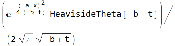
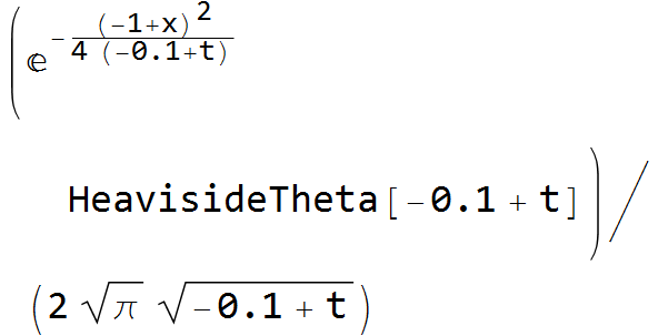
We can choose b to be arbitrarily close to t,
![]()

We can also choose a value of a close to x,
![]()
We can now plot this,
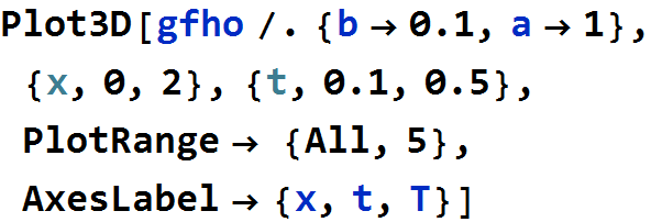
You can see the effect of the Dirac delta, this is why it is called an impulse response.
Using these methods we can get around the issue of infinite densities.
Click here to go back to the quantum mechanics page.
Click here to go back to our home page.