Partial Differential Equations
George E. Hrabovsky
MAST
Introduction
Partial differential equations (PDEs), are much more complicated that ODEs. The goal here is to identify or construct a function of more than one variable that satisfies an equation involving the partial derivatives of a function of more than one variable. We will not attempt any systematic treatment here, and we will more freely use Mathematica than we have until now. The goal is to gain familiarity with how PDEs are written, how boundary conditions are chosen, and how we can solve PDEs using some traditional methods in cooperation with Mathematica.
The General PDEs
Many PDEs of interest are of higher than first-order. Let’s assume a function u(x,y) and a generic homogeneous second-order PDE is
![]()
We choose a trial function f, that is twice differentiable, of the form
![]()
We then find the relevant second-order partial derivatives for our PDE,
![]()
Substituting this into our PDE gives us
![]()
There are three cases we can consider, f''=0, ![]() , or both.
, or both.
If we look at the case f''=0, then we have the solution ![]() . This requires two arbitrary constants instead of two arbitrary functions and is thus not the most general solution. We may thus disregard this as a solution.
. This requires two arbitrary constants instead of two arbitrary functions and is thus not the most general solution. We may thus disregard this as a solution.
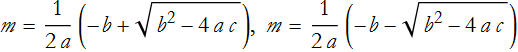
This leads us to consider the case ![]() , where we can choose a linear combination of the variables x and y and get a solution for any twice differentiable function f. This is a quadratic equation leading to the solutions
, where we can choose a linear combination of the variables x and y and get a solution for any twice differentiable function f. This is a quadratic equation leading to the solutions
The sign of the discriminant ![]() is extremely important in determining the number and type of solutions to the quadratic. There are three broad cases
is extremely important in determining the number and type of solutions to the quadratic. There are three broad cases
![]()
In the case ![]() , there are two distinct real solutions. PDEs of this type reduce to the form
, there are two distinct real solutions. PDEs of this type reduce to the form ![]() and are called hyperbolic.
and are called hyperbolic.
In the case ![]() , there is a single degenerate root. PDEs of this type reduce to the form
, there is a single degenerate root. PDEs of this type reduce to the form ![]() and are called parabolic.
and are called parabolic.
In the case ![]() , there are two distinct complex roots. PDEs of this type are called elliptic.
, there are two distinct complex roots. PDEs of this type are called elliptic.
Boundary Conditions
In general all PDEs occur within the infinitude of space. Unfortunately, most applications require the imposition of some geometry. To reflect this we must establish boundaries. If our situation allows for a solution on a circle in any direction, then we impose what we call periodic boundary conditions. An example is the distribution of temperature through a ring.
If there is a boundary where the value of our function u is specified, then we call that a Dirichlet boundary condition, and we call its solution a Dirichlet problem.
If there is a boundary where the value of the normal derivative of our function u' is specified, then we call that a Neumann boundary condition, and we call its solution a Neumann problem.
If there is a boundary where both the value of function u and its normal derivative are specified, then we call that a Cauchy boundary condition, and we call its solution a Cauchy problem.
If there is a boundary where both a linear combination of the values of function u and its normal derivative are specified, then we call that a Robin boundary condition, and we call its solution a Robin problem.
The situation can exist where different boundaries of the same system have different, and disjoint, boundary conditions. Such a situation is called a mixed boundary condition.
The Wave Equation
We can write this important equation,
![]()
where ψ represents a displacement at some position and time and, with given tension T and density ρ, c=T/ρ. This is an example of a hyperbolic equation. The left hand side is the second time-derivative of the displacement, and the right hand side is the Laplacian. In one dimension this becomes
![]()
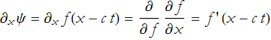
If we think of an arbitrary twice differentiable function, f, and we guess a value of a characteristic curve as the argument of the function,
![]()
then
![]()
![]()
![]()
![]()
![]()
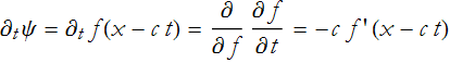
also
![]()
![]()
![]()
![]()
![]()
So (PDE.8) becomes
![]()
the arbitrary function of the characteristic curve will always generate a solution! Magic! Sorcery!
If we accept the D’Alembert solution, then we can write the gene3ral solution as
![]()
We will need to specify the Dirichlet condition
![]()
and the Neumann condition
![]()
We can write this in Mathematica,
![]()
![]()
and then we can use DSolve to solve it,
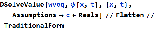
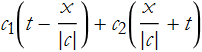
where ![]() is the arbitrary function we called f and
is the arbitrary function we called f and ![]() is g.
is g.
The Heat Equation
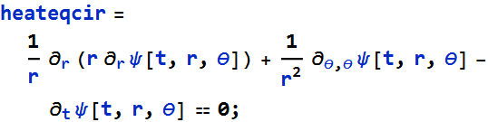
Another important equation is the heat equation, in Mathematica it looks like this,
![]()
![]()
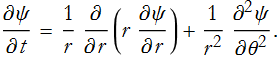
or we can write it traditionally,
![]()
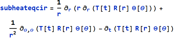
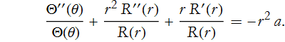
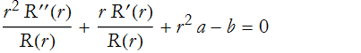
This is an example of a parabolic equation. The following exposition is due to Zwillinger (1992). Let’s say we want to model the heat flow in a circular region. By using polar coordinate we transform (PDE.14) into
We have three independent variables, t, r and θ. We first try to solve this using Mathematica,
![]()
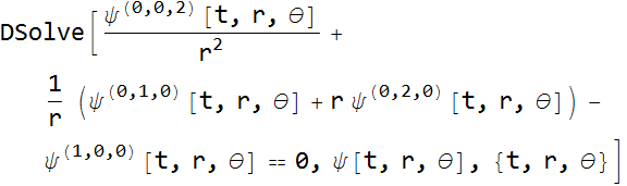
It seems unable to solve this. We could play with some boudnary conditions, but let’s see if we can construct a general solution.
So we construct a product of three functions such that we have a trial form of our solution
![]()
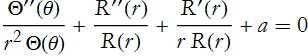
This is called separation of variables. We use Mathematica to substitute this into (PDE.15).
now we make our substitution
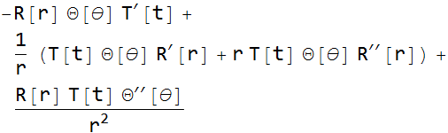
we now try to isolate T[t]
![]()
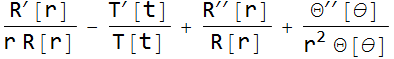
this whole thing is equal to 0
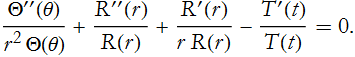
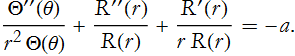
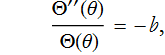
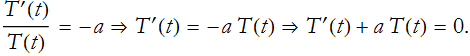
There is only one term that depends on t. Since no other term depends on t, then this term must be constant,
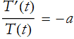
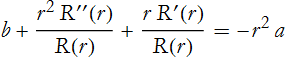
where we use the minus sign for later convenience. We can substitute this into (PDE.17)
There is only one term that needs to be separated, that is the first one,
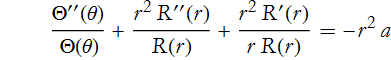
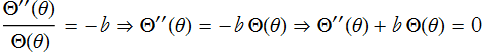
There is now only one term that represents a change in θ. By the same argument as we made for time dependent, we can now make this for θ,
so
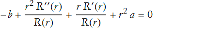
![]()
We have now converted our PDE into a system of ODEs.
![]()
We can now try to solve the first of these with Mathematica,
![]()
![]()
or
![]()
Then we try the second,
![]()
![]()
or
![]()
and
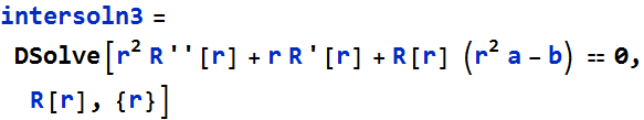
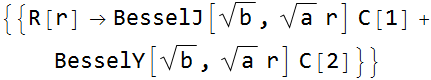
or
![]()
with the Bessel functions J and Y. Of course, we also have five arbitrary constants. Applying this to (PDE.16)
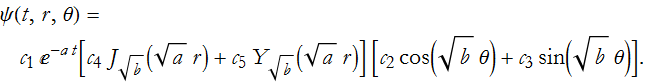
But is this the most general solution? No, the most general solution must occur for all values of a and b, so we need to integrate by these, this is an example of the superposition principle, the sum of solutions form a solution.
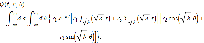
This can be narrowed down by applying conditions based on the physical problem being solved.
Click here to go back to the quantum mechanics page.
Click here to go back to our home page.