Ordinary Differential Equations

George E. Hrabovsky

MAST

Introduction

I am now going to assume that you have solved some equations of motion, or at least you have seen it done. From this it is easy to get the idea that the subject of solving such equations has been laid out in a systematic way and you can start at the beginning and work your way through it. Indeed, there are literally hundreds of books on the subject. It is a huge body of work, most of it assigning classifications and proving that solutions exist. The sad truth is that the collection of solution methods for such equations is an unfinished art-form. The best we can do is show off some of the methods that have been developed and hope we can exploit these ideas to stumble upon our own methods.

Ordinary Differential Equations

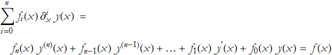
So the central problem is to find one or more functions y(x) that solve an equation having derivatives of y with respect to x..

We denote an m-order derivative of a function, , with special notation for first- and second-order derivatives, respectively, y'(x) and y''(x). If n is the highest order of m, then we say the corresponding differential equation is of order n.

If there is only one independent variable, then we call the equation an ordinary differential equation (ODE). If there is more than one independent variable, we call the equation a partial differential equation (PDE).

If an ODE can be written so that there are specific terms for each order of derivatives, we call it an explicit ODE. If we cannot do this, then we have an implicit ODE.

A linear ODE is explicit,

We can write an operator

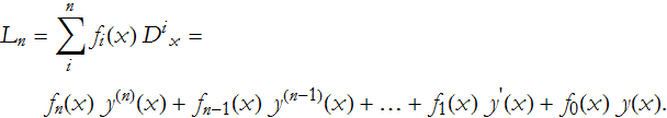
which allows us to write the equation in a much more compact form,

The f(x) in (ODE.1) is called the inhomogeneity of the ODE. If f(x)=0, then there is no inhomogeneity and the equation is said to be homogeneous.

If we have a set of solutions of an ODE, we can form a linear combination of them, just like we did with vectors. Such a linear combination is also a solution of the ODE. If the linear combination is zero when all coefficients are not also zero, then the solutions are linearly dependent, otherwise they are linearly independent. This will become important later.

Theorem ODE-1 For  a homogeneous ODE of nth order, there will be n linearly independent solutions.

If we have a set of n solutions for an nth-order ODE, we will call the linear combination of the solutions a general solution.

Theorem ODE-2: The general solution of a homogeneous ODE of the form will then have the form .

Theorem ODE-3: The general solution of a inhomogeneous ODE of the form will then have the form where is some specific solution.

As an example, we examine the equation describing the harmonic oscillator

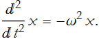
which has the generic form

this has the operator

The general solution is

These parts are linearly independent.

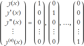
Often we need to associate an nth-order ODE with n initial conditions to find a suitable solution. In general, given the function y(x) we will have the following set of initial conditions

It is easy to show that this fulfills our three theorems above.

There are cases where nonlinear ODEs have solutions that do not appear in the general solution, these are called singular solutions.

What is an Ansatz?

We will introduce something called an ansatz. The word ansatz is German for the phrase, "An initial placement of a tool that works." This is another way of saying that it is a tool that works, but there is no formal justification for it with what we have on hand. We will see this idea used a lot.

Separation of Variables

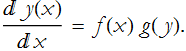
Say that we have a function of an independent variable f(x) and a function of a dependent variable g(y). For an ODE of the form

we will rewrite derivative as

The process of separation, a kind of ansatz for simplifying the ODE, is where we move all like terms to the same side of the equals sign.

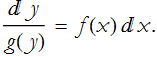
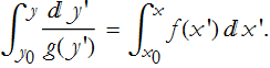
You then integrate both sides.

The Linear ODE with Constant Coefficients

Let’s take a look at the equation of motion for a one-dimensional damped harmonic oscillator. This is, of course, based on Newton’s equation of motion,

The difficulty of Newtonian mechanics is tracking down the expression for all of the Fs. This will be a sum, since forces add like vectors. There is the linear restoring force -k x(t) and then there is the damping force -β x'(t), so we have the second-order linear ODE

We need to figure out what k is, in the absence of friction we could write the initial angular frequency , so , we can also write β=γ m. This gives us the operator equation

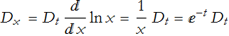
We introduce another ansatz, here we make the substitution . From this we can apply this to our operator equation

where the derivatives are,

so our differential equation becomes the algebraic equation,

this is often called the characteristic equation, or the auxiliary equation. We can then write the solution using the traditional quadratic equation solution

where δ is the discriminant, , it is a nice exercise in algebra to figure out why it has this form.

According to ODE Theorem 2, the general solution will have the form

We have been examining the case where , this is called the aperiodic case (overdamped). It is so-called because the damping is so great that there are no oscillations any more. If then ω=-γ±iδ and we have the underdamped case (here we have an ever deceasing oscillation). We can use Euler’s formula for any choice of δ, and for new constants

So, what about the case where , what we call the critically damped case? Can this result ever really be measured? Probably not precisely. Let’s take this as a limit instead. For this situation we have δ=0, so the roots of our algebraic equation are ω=-γ±0, so we have two equal roots, ω=-γ,-γ. For k repeated roots there is a well-known result,

Thus we have the general solution for this case as

Euler’s Equation 1

This is an equation where each term has a factor of an nth power of the independent variable and a nth order derivative. For example

Euler’s equation has the general form

Since this is homogeneous we can make a substitution,  another ansatz,,

so

this leaves us with the requirement

There are two roots for this equation.

so we have and . By Theorem ODE-2 we then have the general solution

This is called, by some, the power ansatz.

Euler’s and Legendre’s Equation

We will use the same equation as that in the previous section.

Legendre’s equation has a general form

it is easy to see that if k=1 and m=0 that this becomes the Euler equation.

Here we make the substitution . Thus, , we can make a change of variables to simplify our notation, ,

where we make the definition

So,

and

where

so

then

so we have the operator equation

or adopting the change of variables

This is a linear ODE with constant coefficients, which we have already discussed, it has the general solution

Inhomogeneous Linear Equations and Integrating Factors

Given the fact that we know to functions A(x) and B(x), and assuming we have the ODE

We need not specify either of the auxiliary functions. We will need a number of ’s up to the order of our ODE, in this case we need and . To specify it suffices to treat the equation as homogeneous. We thus convert our equation to

divide through by y(x)

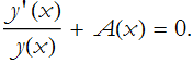
rearrange this a little,

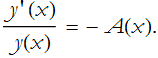
We realize, after staring at this long enough that is a derivative, in this case it is , so we now have,

We can integrate this

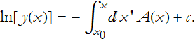
or,

or, since this is a one-parameter, first-order equation,

This is called an integrating factor.

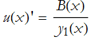
To return to the inhomogeneous case we guess at a new function, we say that . This transforms our equation,

where

or

so

or

we can rearrange this,

We integrate this

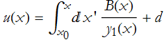
Placing this into our new function we get

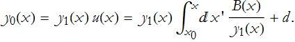
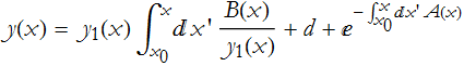
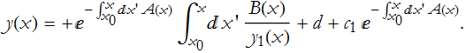
According to ODE Theorem 3, the solution is then

Closing Thoughts

There are many ways to derive and to solve ODEs. There is no systematic way to do this. The more experience you have with various approaches, the more likely you will be to recognize any way to convert your equation into a form to apply a specific method.