Linear Algebra, Part Two: Abstraction

George E. Hrabovsky

MAST

Introduction

It is traditional to introduce vectors as arrows and deduce their properties from a geometrical point of view. In quantum mechanics this point of view is not valid, and we must understand and exploit the abstract nature of vectors.

Vector Spaces

We can formalize the idea of a vector by defining a set, V, as being made of a collection of objects, , , and so on. For now we will not name these objects other than to call them kets. We can add the kets , and we can multiply the kets by a scalar, . We call the set V a vector space if the following tests are all true:

We can define a rule to add the kets.

We can define a rule to multiply a ket by a scalar.

The operation of addition or scalar multiplication results in another object of the set. Another way of saying this is that the proposed vector space is closed under the operations of addition and scalar multiplication.

The addition of kets is commutative. For example, .

The addition of kets is associative. For example,

There exists a null ket, , such that .

For every ket, , there exists an additive inverse ket, such that, .

Scalar multiplication is associative, .

Scalar multiplication is right distributive,

Scalar multiplication is left-distributive,

The kets of the vector space are what we call vectors. In other words, the most general, and useful, definition of a vector is that it is a member of a vector space.

We are using the ket symbol, |V> instead of any of the many more traditional notations for vectors. Why? Because this is an element of the language of quantum mechanics, called the Dirac notation, the details of which we will get to a bit later.

This presentation gives us the ability to examine a lot of structures, of which vector spaces are only one kind.

Algebraic Structures

There is a kind of set that has special properties, a list of structural properties, such as those we listed above for vector spaces. To begin we need to consider a generic set, A, with arbitrary elements, (a,b,c,...), thus we can write . An operation that combines any two elements of a set is called a binary operation. Some examples of binary operations are addition, multiplication, rotation about a point by some specific angle, etc. We symbolize these, . So we have a set with a binary relation. We need another requirement.

If a binary relation, R, is such that a R a holds for every a∈A, then the binary relation is said to be reflexive on A. For example, if we choose the equals sign as the relation symbol, then a = a holds for every element of any set, so equality is reflexive. If a binary relation has the property , then we say that the relation has symmetry. Using our example of equality, a = b implies that b = a, so equality is symmetrical. If a relation has the property that , for all elements , then we say that the relation is transitive. Again using equality we see that if a=b, and b=c, then a=c, thus equality is transitive. Any relation that is reflexive, symmetrical, and transitive is called an equivalence relation, and is denoted with the symbol ~, thus we write, a~b. We can see that equality is an equivalence relation.

Now we can define our special kind of set. We start with a specific set A, a specific binary operation, for example, , and the idea of equality. If all of thse are present we have what we call an algebraic structure. We write such a structure (A,,=).

Structural Properties

You will see that these are just formal statements of the criteria we introduced above.

S1: When binary relations of elements of a set are also elements of the set we say that the set is closed under the binary relation. We can write this

S2: When the order of combinations of actions we take leaves the result unchanged we call that associativity. We can write this,

S3: When we combine a specific element o with any other element of a set that leaves the other element unchanged, then o is called the identity element. We can write this,

S4: When we combine a specific element a with another element -a, if the result is the identity element o, then -a is called the inverse element of a.   We can write this,

S5: When the order of combination of elements under a binary relation doesn’t matter, we call it commutative.   We can write this,

S6: This is a generalization of the familiar right-distributive property.   We can write this,

S7: This is a generalization of the familiar left-distributive property.   We can write this,

We can now construct several common algebraic structures. We begin by defining a generic structure, call it (S,⊕,=).

If S1 and S2 apply, then our algebraic structure is called a semigroup.

If S1, S2, and S3 apply, then we call our algebraic structure a monoid.

If S1, S2, S3, and S4 apply, then we call the algebraic structure a group.

If S1 through S5 apply, then we call the algebraic structure an Abelian group.

These are the structures that come about from a single binary relation.

If we have a set possessing two binary operations, (S,⊕,⊗,=), then we can define a new collection of algebraic structures.

If we have a Abelian group under ⊕, and closure (S1) applies under a second binary operation ⊗, that is both left- and right-distributive (S6 and S7 apply), then the algebraic structure is called a nonassociative ring.

If we have a Abelian group under ⊕, a monoid under ⊗, along with being left- and right-distributive, then the algebraic structure is called a ring with identity.

If we have a Abelian group under ⊕, a monoid under ⊗ along with commutativity (S5), and being left- and right-distributive (S6 and S7), then the algebraic structure is called a commutative ring with identity.

If we have a Abelian group under ⊕, a group under ⊗, and being left- and right-distributive (S6 and S7), then the algebraic structure is called a quotient ring.

If we have a group under ⊕ and ⊗, and being left- and right-distributive (S6 and S7), then the algebraic structure is called a field.

If we have a pair of sets, one set possessing two binary relations, (V,⊕,◦,=), and other also having two binary relations, (F,+,×,=), then we can define another new collection of algebraic structures.

If the structure is written (V,⊕,◦,F,+,×,=), and if this structure forms a ring with identity over ⊕ and ◦, and a field over + and ×, then the structure is called a vector space over the field F.

If we have the structure (V,⊕,A,+,·,◦,=), and if this structure forms an Abelian group over ⊕, an Abelian group over +, a monoid over ·, a group over ◦, and being left- and right-distributive (S6 and S7) for ⊕ and ◦, then the structure is called a module over A.

If we have the structure (V,⊕,⊗,A,+.·,◦,=), and if this structure forms a nonassociative ring over ⊕ and ⊗, a nonassociative ring and S6 and S7 over + and ·, and a group over ◦, and S6 and S7 over ⊕ and ◦, and finally if

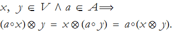
then the structure is called a nonassociative algebra over A.

If we have the structure (V,⊕,A,+,·,◦,=), and if this structure forms a nonassociative ring over ⊕ and ⊗, a ring with identity and S6 and S7 over + and ·, a group over ◦, S6 and S7 over ⊕ and ◦, and S6 and S7over ⊕ and ◦, and finally if Eq. (LA2.8) holds, then this structure is called an algebra with unity over A.

If we have the structure (V,⊕,A,+,·,◦,=), and if this structure forms a nonassociative ring over ⊕ and ⊗, a commutative ring with identity and S6 and S7 over + and ·, a group over ◦, S8 and S9 over ⊕ and ◦, and S6 and S7 over ⊕ and ◦, and—once again—if Eq. (LA2.8) holds, then this structure is called an commutative algebra with unity over A.

The field that we are most familiar with is built out of the set of real numbers and is defined for addition and multiplication, with equality, we write this (R,+,×,=). The most common vector space is the three dimensional Euclidean space with a defined origin, , where is the set of three-dimensional vectors, ⊕ is vector addition, ◦ is multiplication of a vector by a scalar, all of which are defined over the field of real numbers, where the scalars to multiply the vectors are drawn from.

Transformations (Mappings)

The goal of theoretical physics is not just to describe nature, but to provide predictions of how nature functions. To do that we formulate mathematical models. We thus represent physical objects as mathematical objects, like points. We represent physical space by coordinate systems. Changes in the state of an object are represented by transformations of one variable to another. So anything we can do to a transformation can, in some sense, be done to a physical object and/or its state.

We will now explore some properties of transformations in general. We can apply these properties to any transformation. This applies to normal functions, or to derivatives, and so on. These ideas are abstract, that is their power.

We can define any given transformation as a rule that causes something to change into something else. A transformation, f, takes an element of one set, say X, and changes it into an element of another set, say Y. This is often symbolized,

or,

There are several names for transformations that are equivalent: function, mapping, and morphism.

The first property of a transformation is that the elements of the set that it transforms is called the domain of the transformation. More formally, the domain of a transformation is a set of elements,

So assuming that the transformation turns every value of x into some value of y, the set of possible x values is the domain.

We can also establish the range as the set of values the x element is converted into,

The set from which the values of the range are drawn from is called the codomain.

A transformation whose range is the whole codomain, ran(f)=Y, is called a surjection—or it is said to be onto.

If every pair of unequal elements produces unequal transformations,

then the transformation is called an injection, or it is said to one-to-one. Any transformation that is both an injection and a surjection is called a bijection, or it is in one-to-one correspondence.

If we treat one transformation as dependent upon another transformation, we say they are composed. We treat one transformation, say the function g(x) as the argument of another, say f(x), then we write f(g(x)), or, if f:X→Y and g:Y→Z then the composition is g◦f:X→Z. The chain rule for differentiation is a good example of this.

Vector Spaces II

We can think of a vector space as a set of vectors that form an Abelian group under addition and a group under multiplication by a scalar, where the scalars are the elements of a specific field, and where vector addition and scalar multiplication are both left- and right-distributive.

The first example we will mention is . This is the vector space of all nth-order column matrices, , along with the binary operations of column matrix addition and multiplication by a scalar. This becomes a vector space when we choose a reference point to be an origin, however temporarily. Here the set of real numbers, R, is the underlying field, along with the binary operations of addition and multiplication.

Another example of a vector space is given by . This is the vector space space of all n-tuples (row matrices): . Here F is an arbitrary algebraic field. We have the first binary operation of addition of n-tuples,

The second binary operation is scalar multiplication where an n-tuple can be multiplied by a scalar, term by term,

A third example is (P(t),+,·,F,+,·,=) The set of all polynomials of order n where the polynomials, , are the vectors. Here F is an arbitrary field from which the coefficients are drawn. Vector addition is just the sum of the polynomials. Scalar multiplication is the product of a polynomial by some number drawn from F.

A fourth example is (A,+,·,F,+,·,=) the set of all matrices A of a given order in m and n, 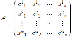where each matrix is an individual vector. Here F is an arbitrary field. The first binary operation is just the addition of matrices. Scalar multiplication is just the multiplication of the matrix by an element of F.

The fifth example of a vector space is (T(x),+,·,F,+,·,=) the set of all functions, T:X→F, where the individual functions are the vectors. The set F is an arbitrary field. Vector addition is the sum of two functions, (f+g)(x)=f(x)+g(x). Scalar multiplication is just the product of a function and an element of F, (c f)(x)=c f(x).

The sixth example is (D(x),+,·,F,+,·,=), the space of all differentiable functions, where the differentiable functions are the individual vectors. The set F is an arbitrary field. The first binary operation is an expression of the sum rule of differentiation, D(x+y)=D(x) + D(y). The second binary operation is an expression of the constant multiple rule, D(a·x)=a·D(x).

Any subset S of a vector space that is also a vector space is called a subspace of V. The intersection of any number of subspaces of a vector space is also a subspace of the vector space.

If a set of vectors can be written as a sum of products of coefficents

we call this a linear combination.

If such a linear combination of basis vectors forms the null vector for some set of coefficients (not all equal to zero)

then the basis vectors are linearly dependent. Thus, one of the vectors is the sum of all of the others. If a set of vectors is not linearly dependent, then it is said to be linearly independent.

If we have a linearly independent combination of basis vectors and coefficients

then the set of basis vectors, , are said to span the vector space. Here and , the underlying field.

Linear Transformations

Linear problems are the only ones that we can usually solve directly. So we use these kinds of transformations all the time. We can even approximate nonlinear problems using linear methods.

We now can state that any transformation from one vector space to another,

such that for any scalars and any vectors , we have,

is called a linear transformation.

The set of elements that map into the zero vector of W is called the kernel of the linear transformation,

The set of points in W mapped by T from V is called the image of T,

The kernel and image of a linear transformation T, ker(T) and im(T), are both subspaces of V.

The dimension of a vector space is the sum of the dimensions of the kernel and image.

Any linear transformation that is a bijection is also called a isomorphism.

A linear transformation from a vector space into itself is called a linear operator,

A transformation I that operates on another transformation T that leaves T unchanged is called the identity transformation,

A transformation that gives the identity transformation when applied to T, is called the inverse transformation,

Representing a Linear Transformation by a Matrix

In order to represent a linear transformation,

as a matrix we need to do several things:

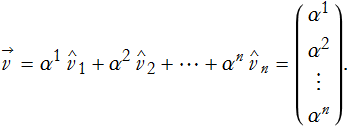
Fix a basis for V, . We can write any vector that is an element of V as a linear combination,

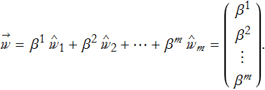
Fix a basis for W, . Similarly we can write any vector that is an element of W as a linear combination,

In order to transform one column vector into another column vector requires a transformation matrix. In this case the transformation converts into . For this choice of basis, we have,

We can expand this out,

We can define the action of the transformation on a given component of a vector as,

From this we can see that the transformation matrix will be,

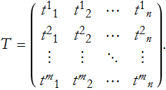
Given the transformation matrix T, the linear transformation acts on the vector v like this,

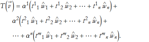
So, the linear transformation can be represented by a matrix.

Click here to go back to the quantum mechanics page.

Click here to go back to our home page.