Linear Algebra, Part One: Matrices

George E. Hrabovsky

MAST

Introduction

The language of quantum mechanics is often that of linear algebra. There are two main views of linear algebra (okay, three, but modules are too advanced for now). One is based on abstract vector spaces and the other are matrices. There is an important principle that tells us both are identical. We will start with matrices as they allow us to make calculations.

Matrices

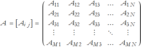
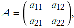
A matrix is a rectangular array of real or complex numbers. We say that there are M rows and N columns of a matrix. The number of rows and columns form the order of the matrix. We can also call it an M×N matrix. If the matrix is labeled A, then we will have elements labeled by column and row as indices, , where i=1,…,M and j=1,…,N.

You might also see the elements of a matrix in the form , , or . For us this is not impiortant, we will use subscripts. There are times when this placement is very important, so be sure you know what context you are working in.

A matrix having one row and N columns, is a row matrix

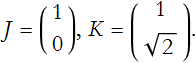
A matrix having M rows and a single column, is a column matrix

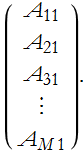
A matrix having the same number of rows and columns is called an N × N square matrix.

Basic Matrix Arithmetic

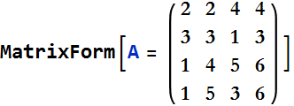
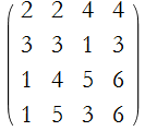
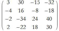
For the exercises that follow we will use the following matrices:

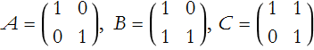
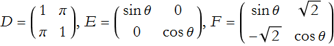
If two matrices, say O and P, have the same elements then they are equal and we write O = P.

We can add two matrices by adding their elements,

LA1-1: Add A to the matrices B through F.

We can also subtract two matrices by subtracting their elements,

In order to add or subtract matrices they must be of the same order, another word for this is conformable.

We can multiply a matrix by a number, say a, by multiplying each element by a,

In this way we can change the sign of a matrix,

The following rules apply, first addition is commutative,

Addition is associative,

There is an additive identity, in this case it is a matrix all of whose elements are 0, we will label this 0,

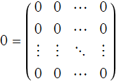
so

There is an additive inverse,

Multiplication by a number is right-distributive,

Multiplication by a number is also left-distributive,

Matrix Multiplication

Given two matrices, R and S, where R is an M ×N matrix and S is an N × T matrix the matrix product of the two is

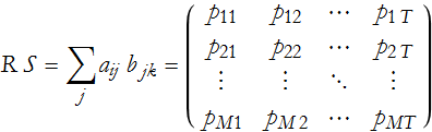
where i=1,…,M, j=1,…N, and k=1,…,T. Where the elements are a set of products,

Assuming all matrices are conformable, then the matrix product is left- and right-distributive and associative

In general, the matrix product is not commutative.

In general, O P=0, does not imply that either O=0 or that P=0.

In general, A B=A C does not imply that B=C.

LA1-2: Multiply B to the matrices B through F and then reverse the multiplication.

Special Matrices I

We now introduce five important kinds of matrices.

A square matrix with all off-diagonal elements zero, an all diagonal elements non-zero is called a diagonal matrix.

A diagonal matrix whose diagonal elements are all 1, is called the identity matrix, and is denoted I.

A square matrix whose elements satisfy the condition , is called an upper triangular matrix.

A square matrix whose elements satisfy the condition , is called a lower triangular matrix. Another way of defining a diagonal matrix is that it is both upper and lower triangular.

Matrix Inverses

If O P=I=P O, then P is the inverse matrix of O, .

We also note that .

Similarly .

In general, for a 2 × 2 matrix

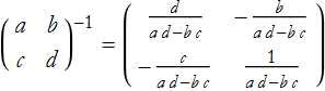
LA1-3: Find the inverse matrices A through F.

Matrix Transpose

A matrix that is the interchange of rows and columns is the transpose of the matrix. We denote this with a T superscript,

The following rules hold.

Special Matrices II

A matrix equal to its transpose is called symmetric, .

A matrix equal to its negative transpose is called skew-symmetric, .

Determinants

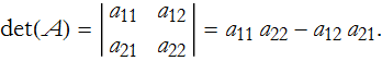
A determinant is a special kind of function that takes a matrix and converts it into a scalar. We will begin with notation, the determinant of a matrix, A is denoted either det(A), or . So, what is a determinant? We will begin with the simplest matrix,

then the determinant is said to be of first order and is written,

Interesting result, but not very revealing.

Let's look at an arbitrary 2×2 matrix,

this determinant is said to be of second order,

We can see how this structure comes about be examining the array,

here you can see that the first term in (25) is given by multiplying the diagonal elements of the array from the upper + side. The second term in (25) is given by subtracting the diagonal terms from the upper - side, then keeping the negative sign, thus we subtract the second term.

This gives us a better clue about how to proceed. We can extend this to an arbitrary 3×3 matrix,

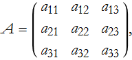
then the determinant is,

We can look at the array and see geometrically how we combined elements,

here we have the first positive term, . We can also construct the next positive term,

. We can then construction the final positive term,

. We can also construct the first negative term,

. Then we have the second negative term,

. Then we have the last negative term,

. If we look at (27) long enough we will notice that we can factor it a bit,

Something interesting is happening here. If we convert the differences into lower-order determinants,

The first determinant is gained by eliminating row 1 and column 1, the indices of the coefficient of the determinant,

the second determinant is gained by eliminating row 1 and column 2,

the final determinant is gained by eliminating row 1 and column 3,

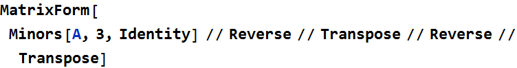
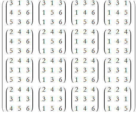
Here we note that we have made three submatrices whose determinants are of order -1 from the order of the original matrix. Such a determinant is called a minor of the element , where we have eliminated row i and column j. We can denote the minor as . So  given (4) we can find the minor of an element, . We first eliminate the 3rd row and then the first column,

this gives us,

In this way we can actually calculate the elements of the determinant. If we consider the sign of the minor, then we can define the cofactor of the element as,

Using our example above we find the cofactor for ,

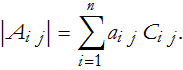
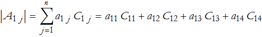
We can now write the determinant as the sum of the products of the elements of any row or column and their respective cofactors. For the ith row we have,

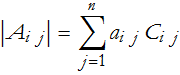
for the jth column,

These are called the Laplace expansions of the determinant. Here is a numerical example,

Step 1: Choose an element, say . In our example .

Step 2: Eliminate the rows and columns associated with our choice. In our case we remove the first row and the first column,

giving us the minor for ,

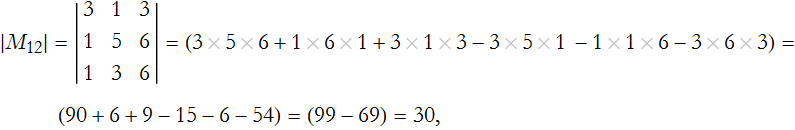
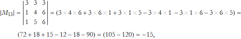
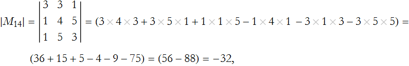
Step 3: Determine the relevant cofactor,

Step 4: Expand through each element using (29) or (30),

Cramer’s Rule

One application of determinants is finding the solution of a matrix equation. If we have a square matrix A, and two column matrices x and b,

we can solve for the ith component of x,

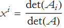
where is the matrix formed by removing the ith column of A and substituting b.

Adjoints

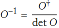
The transpose of a matrix of the complex conjugates of a matrix is called the adjoint of the matrix and is written . A matrix that is equal to its adjoint is called Hermitian. The adjoint is sometimes called the Hermitian conjugate.

If a matrix has a non-zero determinant, then

Eigenvalues and Eigenvectors

Let’s say we have a square matrix O, a column matrix x, and a number λ. Consider the matrix equation

we can rewrite this

We can then solve this equation. The most obvious solution occurs when x is the zero column matrix, this is the trivial solution. Nontrivial solutions exist when

This is the characteristic equation of O.

We can expand this into a characteristic polynomial in λ of degree n,

thus having n roots. The roots of the characteristic polynomial are the set of eigenvalues of the matrix that satisfy the equation (LA1.38). A solution of (LA1.37) in the form of a value for the column matrix will exist for every eigenvalue and is called an eigenvector.

LA1-4: Find the eigenvalues of the matrices A through F.

LA1-5: Find the eigenvectors of the matrices A through F.

Click here to go back to the quantum mechanics page.

Click here to go back to our home page.