 , is neither true nor false as it is presented. It becomes a proposition only if we define x in some way. We need to develop a couple of additional ideas.
Day 2: Logic and Proof
George E. Hrabovsky
MAST
This is the second installment of the series. Here I intend to present the ideas and methods of proof.
To begin with, I will need to present the basic method of mathematics. I will try to make this as simple as possible and still be useful. It is important to realize that in mathematics, until an idea is applied to something concrete, ideas have no meaning. Thus mathematics is the ultimate abstraction from reality; we speak of pure ideas without regard to meaning. It is best to think of mathematics at this level as a kind of structure.
To succeed in mathematics we need to consider several different notions:
In the table below you will find definitions and examples of the operations of the logic of propositions. It will be understood that a proposition will be symbolized as p, q, r, s, .... All of these symbols may be used in proofs.
| PropositionalOperation | Symbol | Meaning | Eaxample |
| Negation | ¬ | Not | ¬p |
| Conjunction | ∧ | This And That | p ∧ q |
| Disjunction | ∨ | This Or That | p ∨ q |
| Exclusive Disjunction | ⊻ | This Or That But Not Both | p ⊻ q |
| Conditional | ⇒ | If p, Then q | p⇒q |
| Converse | ⇒ | The Converse of If p, Then qis If q, Then p. | q⇒p |
| Contrapositive | ⇒ | The Contrapositive of If p, Then q is If Not-q,Then Not-p. | ¬q⇒¬p |
| Bicondictional | ⇔ | p If and Only Ifq. If and only if, is sometimeswritten iff. | p ⇔ q |
From these symbols we can create logical formulas. The simplest formula is just the statement of a proposition, for example p, or if we are making a statement that a proposition p depends on another idea, say x we would write p(x).
Every proposition, indeed every logical formula, is either true or false. We can create a table of these values using T for true, and F for false. When we make this array using all possible truth values, we call it a truth table. For example, we can create the truth table for the negation of a proposition p:
p
¬p
T
F
F
T
Here is the truth table for the conjunction between two propositions p and q, where we list all possible truth values of the propositions and apply the definition of the conjunction to determine the resulting truth value.
p
q
p ∧ q
T
T
T
F
T
F
T
F
F
F
F
F
Here is the truth table for a somewhat complicated formula:
p
q
r
p ∧ q
¬r
(p ∧ q) ∨ ¬ r
T
T
T
T
F
T
F
T
T
F
F
F
T
T
F
T
T
T
F
T
F
F
T
T
T
F
T
F
F
F
F
F
T
F
F
F
T
F
F
F
T
T
F
F
F
F
T
T
If two formulas have the same truth table result, then they are said to be logically equivalent. We would write p~q if p and q are logically equivalent. If a formula is always true, then it is called a tautology. If a formula is always false, then it is called a contradiction.
The language of modern mathematics is a combination of logic and set theory. We understand a set to be a collection of objects of some kind. Here is a table of basic ideas from set theory.
| Idea | Symbol | Meaning |
| Element of a Set | x∈X | x is an element of the set X. |
| Subset of a Set | X⊆Y | The set Xis a subset of the set Y if every element of Xis also an element of Y. |
| Equal Sets | X=Y | The set Xis equal to the set Y if every element of X is also an element of Yand every element of Y is also an element of X. |
| Unequal Sets | X≠Y | X and Yare not equal. |
| Proper Subset | X⊂Y | X⊆Yand X≠Y. |
Not all mathematical statements are propositions. Indeed, , is neither true nor false as it is presented. It becomes a proposition only if we define x in some way. We need to develop a couple of additional ideas.
In what follows, we will identify the starting proposition, the given, as the hypothesis and symbolize it by p. The conjecture to be proved, the conclusion, will be symbolized by q.
This is the most rudimentary style of proof. The primary limitation is the amount of work it requires, and the ever-expanding size of the resulting truth table. You begin by producing the truth table for the hypothesis, and then the conclusion; if they are the same, then they are logically equivalent, thus the hypothesis iff the conclusion.
This is at once the most effective proof and the most difficult. Here are the steps:
State the hypothesis.
Make your first argument in a sequence that will bring you to the conclusion.
: (this symbol indicates a variable number of steps).
Make you final argument.
State your conclusion.
Often this process is ended by writing Q.E.D. standing for qoud erat demonstratum, meaning roughly, "Which was to be demonstrated."
The contrapositive and the conditional are logically equivalent, thus if we can prove the contrapositive, we have proven the conditional. We begin this method of proof by stating the conclusion.
State the conclusion.
Write the negation of the conclusion.
Make your first argument in a sequence that will bring you to the hypothesis.
:.
Make your final argument.
State the negation of the hypothesis.
Make the argument that by the contrapositive the conditional must be true. Q.E.D.
I gave Galileo's example of this type of proof in the Day One Theoretical Physics Article.
State the hypothesis.
Assume that the hypothesis implies the negation of the conclusion
Make your first argument in a sequence that will bring you to the conclusion.
:.
Make you final argument.
Show that this implies that the negation of the conclusion is both true and false, such a situation is always false.
Since this a contradiction, the negation of the conclusion cannot be true.
The conclusion must then be true. Q.E.D.
This requires knowing that the natural numbers are 1, 2, 3, and so on.
State the hypothesis.
Show that the conclusion is true for the case of a variable equal to one. This is called the basis step.
Write your conclusion for the variable having an arbitrary value for some unspecified natural number n.
Show that if the conclusion is true for n that the conclusion is also true for n+1. This is called the inductive step. It is possible to reverse 3 and 4, to assume the conclusion true for n+1 and then show that it is true for n.
By the Principle of Mathematical Induction the conclusion must be true for all natural numbers (or for all cases that can be listed by the natural numbers). Q.E.D.
The final style of proof is given in the next two sections:
State the hypothesis.
Show that the conclusion requires a finite number of cases.
Prove each case independently.
Thus the conclusion is true for each possible case. Q.E.D.
We continue with the second method for case analysis:
State the hypothesis.
Show that the conclusion requires a finite number of cases.
Prove the first case.
Prove each case based on the proof of the previous case.
Thus the conclusion is true for each case. Q.E.D.
Up to now we have considered how to construct a mathematical proof. We can also disprove a conjecture by showing a single case where the conclusion is not true. Such an instance is called a counterexample of the conjecture.
Using [1] as a basis, I will begin with some logical operations.
| Operation | Mathematica Command | Explanation |
| Negation | ! expression | Negates the expression. |
| Conjunction | e1 &&e2 &&... | Returns True if e1 and e2 aretrue, otherwise it returnsFalse. |
| Disjunction | e1 || e2 || ... | Returns True if e1 or e2 aretrue, otherwise it returnsFalse. |
| ExclusiveDisjunction | Xor[e1,e2,...] | Returns True if either e1 ore2 are true, but not both, otherwise it returns false. |
| Conditional | Implies[p,q] | This represents theconditional p ⇒ q. |
| Biconditional | Equivalent[p,q] | This represents thebiconditional p ⇔ q. |
| ForAll | ForAll[x,expr] | This is the universalquantifier. |
| Exists | Exists[x,expr] | This is the existentialquantifier. |
We can use Mathematica to develop truth tables. We will first use the command BooleanTable[logical expression,{logical variable 1},{logical variable 2}, ...]
![]()
![]()
We can put this into the form of a table by either wrapping the function in TableForm[],
![]()
| True | False |
| False | False |
or by adding //TableForm on the end
![]()
| True | False |
| False | False |
We can make it numerical, where 1 stands for True and 0 for False by Wrapping the command in Boole[ ].
![]()
| 1 | 0 |
| 0 | 0 |
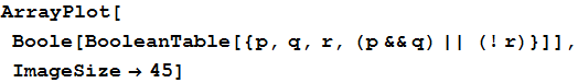
We can even make a pictogram of the truth table by wrapping the command in ArrayPlot. Here the black squares represent the value True and the white the value False.
![]()

We can make the image smaller by specifying an ImageSize->45
![]()

Here is the picture of a truth table for a more complicated formula,
![]()
| True | True | True | True |
| True | True | False | True |
| True | False | True | False |
| True | False | False | True |
| False | True | True | False |
| False | True | False | True |
| False | False | True | False |
| False | False | False | True |
Or graphically,

In this way it is easy to see logical equivalence and to use truth tables to prove logical statements.
The following are arguments of logic. It is a useful exercise to prove each of these, either by writing their truth tables, or by other methods.
| Argument | Name | Formula | Explanation |
| 1 | Definition of aContradiction | (p ∧ ¬ p)⇒F | A proposition and its negation cannot both be true. |
| 2 | Definition of a DoubleNegative | ¬(¬p)⇒p | The negation of a negation of a proposition is the proposition. |
| 3 | Law of theExcludedMiddle | (p ∨ ¬ p) | Either something is true or it is not. This is similar to argument 1. |
| 4 | Definition of Commutation | (p * q)⇔(q*p) | This is true when you replace * with either ∧ or ∨. |
| 5 | Definition of Associativity | (p*q)*r⇔p*(q*r) | This is true when you replace * with either ∧ or ∨. |
| 6 | Law of theContrapositive | (p⇒q)⇔(¬ q⇒¬ p) | This is the basis for proof by contrapositive. |
| 7 | DeMorgan'sLaws | ¬ (p * q)⇔ (¬p ◦ ¬q) |
This is true when you replace * with either ∧ or ∨ and ◦ with either∨ or ∧, respectively. |
| 8 | Definition of a Distribution | p*(q◦r)⇔ (p*q)◦(p*r) |
This is true when you replace * with either ∧ or ∨and ◦ with either ∨ or ∧, respectively. |
Proof: Here is an example of a proof by truth table, we will prove Argument 1, Contradiction.
p
¬p
(p ∧ ¬ p)
Contradiction
T
F
F
F
F
T
F
F
thus (p ∧ ¬ p)~Contradiction, which proves argument 1. QED.
Here is an example of how to discover a proof. We will prove Argument 2, Double Negative. We need to show that the double negative is equivalent to the initial proposition.
We start by stating that the negation of a proposition always has the opposite truth value of a proposition, thus we can write
![]()
The negation of q will then have the opposite truth value from q, we can write,
![]()
Since a proposition is either true or false, when a negation is false the starting proposition is true.
When r is false, then q must be true, this also means that p is false.
Similarly when r is true q is false, and thus p is true.
Therefore we see that r and p are the same.
Since r is the double negative of p, then we can say that the double negative of any proposition is the same as the proposition. This has been a proof by cases. QED.
In [5] we explored the idea of a limit. We begin with the formal definition of the limit:
Definition 1 The Limit: The limit of some function f(x) as x approaches some specific value a is symbolized by
![]()
so long as we make f(x) get as close to L as we want such that x is sufficiently close to a and so long as x never really becomes a.
While this definition is adequate, it will eventually be replaced by a more accurate one.
| Argument | Name | Formula | Explanation |
| 9 | Constant Multiple Rule forLimits |  |
The limit of a constant multiple of a function is the constantmultiple of the limit. |
| 10 | Sum and DifferenceRulefor Limits | 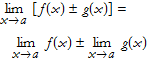 |
The limit of a sum is the sum ofthe limits. |
| 11 | ProductRule forLimits | 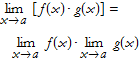 |
The limit of a product is the product of the limits. |
| 12 | Quotient Rule forLimits | The limit of a quotient is the quotient of the limits. | |
| 13 | Power Rule for Limits |  |
The limit of a power is the powerof the limit. |
| 14 | Root Rule for Limits | 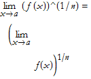 |
The limit of an nth root is thenth root of the limit. |
| 15 | Constant Limit Rule | The limit of a constant is thatconstant. | |
| 16 | Limiting Value | ||
| 17 | Power of a LimitingValue | ||
| 18 | Limit of a Polynomialp(x) | ||
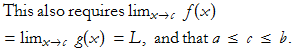
| 19 | Limit Theorem 1 | f(x)≤g(x) ⇒ |
For allxon an interval [a,b]where a≤c≤b. |
| 20 | Squeeze Theorem | If f(x)≤h(x)≤g(x), then |
 |
| 21 | Infinite Limit | This is written if and only if we can make f(x) arbitrarily largefor all values of x sufficiently close to aso long as x ≠ a. | |
| 22 | Negative InfiniteLimit | This is written if and only if wecan make f(x) arbitrarily large and negative for all values of x sufficiently close to a so long as x ≠ a. | |
| 23 | Limits at Infinity | Infinity and zero can be thought of as inverses. | |
| 24 | Infinite PolynomialLimit | 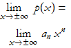 |
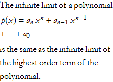 |
| 25 | Continuous Functions | A function is continuous, or smooth,if at any point a thelimit of the function is the limitat that point. | |
| 26 | Intermediate ValueTheorem (IVT) | If f (x) is continuous on an interval [a, b] , and if n is anumber such that f (a) ≤ n ≤ f (b), then there exists some number csuch that, a < c < b,and f (c) = n. | This is a special way of saying that every continuous function will take on all values between f (a) and f (b). |
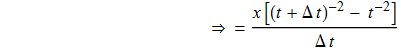
Here is a proof of Argument 15, The Constant Multiple Rule for Limits. For this we immediately require a more precise definition of the limit than the one we have above. We need to define the absolute value,
![]()
eqn 1
So, we redefine the limit,
Definition 1a: The Limit. For some function f(x) then
![]()
if (∀ε)(ε>0) (∃ δ)(δ>0)
![]()
whenever
![]()
Proof of Argument 15: To accomplish this proof we need to show that the limit of the constant multiple of an arbitrary function is the same as the constant multiple of the limit of the function. It seems the most straightforward way to do this is to compute both expressions and show they are equivalent.
Let us begin with the hypothesis, ![]() .
.
By the definition we have some value ε>0 such that
![]()
eqn 2
whenever there is a value δ>0 such that,
![]()
If we think about this for a while we realize that in this situation the limit L is the product of a different limit M and the constant c, by the definition of the limit.
This gives us a nice clue as to how to complete the proof; we need to show that (2) is equivalent to |c| |f(x) - L | < ε.
We begin by rewriting (2)
![]()
By argument 35, (the distributive property) we can rewrite this,
![]()
eqn 3
So, by (1) we have ![]() , and by (3) we have
, and by (3) we have ![]() .
.
Thus we have ![]() , QED.
, QED.
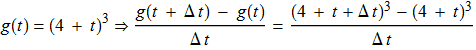
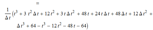
In [5] I introduced the idea of differential calculus. We will present the following definition of the derivative of a function:
Definition 2 The Derivative: The derivative of a function, f(t) is given as,
![]()
| Argument | Name | Formula | Explanation |
| 27 | Differentiability | A function is differentiable atsome point a if f' (a) exists. | |
| 28 | Differentiabilityon an Interval | A function is differentiable on aninterval [a,b] if f' (t) exists for every point a≤t≤b. | |
| 29 | Continuity | If f (t) is differentiable at t = a,then f (t) is continuous at t = a. | |
| 30 | Slope of aTangentLine | The slope of a line tangent to a point a on f (t) is f' (a). | |
| 31 | Constant DerivativeRule | The derivative of a constant is 0. | |
| 32 | ConstantMultipleRule | The derivative of a constantmultiple is the constant multiple of the derivative. | |
| 33 | Sum Rule | [f(t) ± g(t)]'=f'(t) ± g'(t) | The derivative of a sum is thesum of the derivatives. |
| 34 | Power Rule | ||
| 35 | Product Rule | [f(t) · g(t)]'=f'(t) g(t)+ g'(t) f(t) | |
| 36 | Quotient Rule | 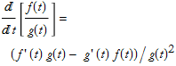 |
|
| 37 | Chain Rule | This allows you to change variables in differentiation. It is a direct application of argument11, above. |
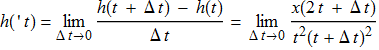
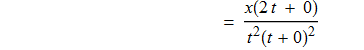
I will now prove Argument 32, The Constant Multiple Rule. We begin with the hypothesis.
Assume that we have ![]() .
.
By Definition 2, this gives us, ![]()
Factoring this we have, ![]()
Then by Argument 36, The Constant Multiple Rule for Limits, we now have, ![]()
This is equivalent, by the definition of the derivative, to ![]() , the conclusion.
, the conclusion.
Thus ![]() =
=![]() , QED.
, QED.
In [5] I introduced the idea of an integral. Given any function f(t), its antiderivative is the function F(t) such that,
![]()
The most general antiderivative is called the indefinite integral and is written,
![]()
Here are some arguments involving integration.
| Argument | Name | Formula | Explanation |
| 38 | Constant MultipleRule | ∫k f(t)dt=k∫f(t)dt | This allows us to factor anymultiplicative constants out ofthe integrand. |
| 39 | Sum Rule forIntegrals | ∫f(t)±g(t)dt=∫f(t)dt±∫g(t)dt | The integral of the sum is thesum of the integrals. |
| 40 | Power Rule forIntegrals | Here n≠-1. | |
| 41 | Constant Rule forIntegrals | ∫kdt=k t + c | |
| 42 | Substitution Rule | 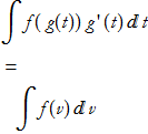 |
Here we understand thatv = g(t). This is an applicationof the Chain Rule,(Argument 37) above. |
| 43 | FundamentalTheorem of Calculus | 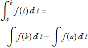 |
In essence this defines anintegral over an interval from ato b. Such an integral is called adefinite integral. The values aand b are called the limits ofintegration. |
| 44 | Interchanging the Limits of ntegration | We can interchange the limits of integration by changing the sign. | |
| 45 | The Same Limits | ||
| 46 | Splitting the Limitsof ntegration | 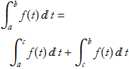 |
We can split the limits of integration so long as a≤c≤b. |
| 47 | Equivalent Integrals | ||
| 48 | ConstantRule forDefinite Integrals |
I will prove Argument 38, the Constant Multiple Rule for Integration. Here we begin with the definition of the integral.
By the definition of an integral∫f(t)dt=F(t) + c.
This implies [F(t) + c]'=f(t).
By argument 32 we can multiply this by an constant k, k [F(t) + c]'= k f(t).
We can apply this to step 1 and get, ∫k f(t)dt=k F(t) + k c.
By argument xx, The Distributive Property, the right hand side of this becomes, k F(t) + k c=k [F(t) + c].
By the definition of integration this is equivalent to k∫f(t)dt=k[F(t) + c].
By step 5 then ∫k f(t)dt= k∫f(t)dt. QED.
In [5] I introduced the idea of a series. Here I formalize that. I will make three definitions.
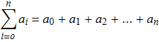
Definition 3 Sequences: A sequence is a list, in a specific order, of n terms. A sequence is called infinite if n→∞. A sequence may be writeen,
![]()
Definition 4 Limit of a Sequence: An infinite sequence {s(n)} has a limit
![]()
if, ∀p>0, ∃N such that ![]() for n>N.
for n>N.
Definition 5 Series: A series is the sum of the first n terms of a sequence.
If this is the sum of an infinite sequence, then it is called an infinite series.
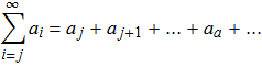
Definition 6 Sequence of Partial Sums: Associated with every infinite series is the sum of the first n terms of the infinite series
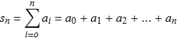
This is called the sequence of partial sums ![]() .
.
| Argument | Name | Formula | Explanation |
| 49 | Convergent sequence | A sequence that has a limit issaid to converge. | |
| 50 | Divergent sequence | A sequence that does not converge is said to diverge. | |
| 51 | Relevance oflimit theorems | The arguments relating limitsare applicable to the limits of sequences. | |
| 52 | Bounded above | A sequence is bounded above if every value of the sequence isless than some value of B. B iscalled the upper bound. | |
| 53 | Bounded below | A sequence is bounded below if every value of the sequence is more than some value of B. B iscalled the lower bound. | |
| 54 | Monotone nondecreasing | Every subsequent term of thesequence is less than, or equalto, the previous term. | |
| 55 | Monotone strictly increasing | Every subsequent term of thesequence is less than theprevious term. | |
| 56 | Monotone nonincreasing | Every subsequent term of thesequence is greater than, orequal to, the previous term. | |
| 57 | Monotone strictly decreasing | Every subsequent term of thesequence is greater than theprevious term. | |
| 58 | Convergence of monotonic sequences | An infinite sequence that isbounded from above and ismononotic nondecreasing isconvergent. Likewise an infinitesequence that is bounded fromabove and is monotonic frombelow is convergent. | |
| 59 | Least upper bound axiom | 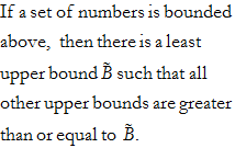 |
|
| 60 | Greatest lower bound theorem | 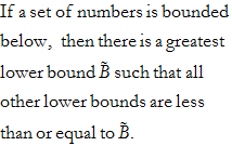 |
|
| 61 | Proper divergence | A sequence that tends to infinityor negative infinity is divergent. | |
| 62 | Oscillating sequences | A sequences that diverges, but is not properly divergent, iscalled oscillatory. | |
| 63 | Monotonic sequences and convergence/divergence | A monotonic sequence either converges or is proper divergent. | |
| 64 | Subsequence | If we can define a new infinitesequence from a given sequence by ignoring some terms we have a subsequence. | |
| 65 | Limit of a subsequence | 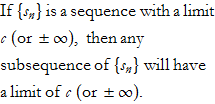 |
|
| 66 | Oscillatory subsequences | A sequence with two subsequences that have different limits is oscillatory. | |
| 67 | Limit of a subsequence of a monotonic sequence | 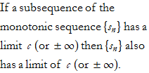 |
|
| 68 | Cauchy condition | 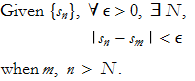 |
Far out in the sequence, all terms are close together. |
| 69 | Cauchy criterion | If a sequence converges then itsatisfied the Cauchy condition, also if the sequence satisfies theCauchy condition it isconvergent. | |
| 70 | Convergence of infinite series | An infinite series converges if its sequence of partial sums is bounded. | |
| 71 | Proper divergence of an infinite series | An infinite series is properdivergent if its sequence of partial sums is unbounded. | |
| 72 | Oscillating infinite series | An infinite series is oscillating if its sequence of partial sums isoscillatory. | |
| 73 | Zero terms | Adding or removing zero termsto a series has no effect on theseries. | |
| 74 | Replacement of k terms in an infinite series | 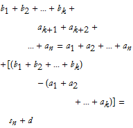 |
The effect of replacing terms in an infinite series is to add a constant to the nth partial sum of the original series. In general this leaves the convergence ofthe original series unchanged. |
| 75 | 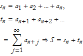 |
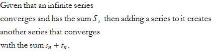 |
|
| 76 | 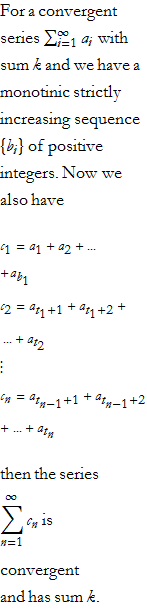 |
The converse of this is not true. We can also say that if, after parenthesis are insertedinto a given series, the newseries diverges, then the originalseries diverges. | |
| 77 | Multiplication of a series by a constant |  If then 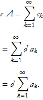 |
|
| 78 | Sum of series | 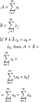 |
|
| 79 | Cauchy criterion for infinite series | ∀ε>0, 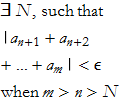 |
Thi is Argument 69 rewritten for infinite series. |
| 80 | Dominated Series | 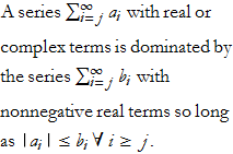 |
|
| 81 | 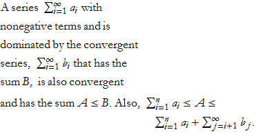 |
Continue building your library of references. Definitely begin with references [3] and [4].
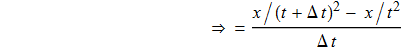
![]()
![]()
and
![]()
![]()
thus the three functions become,

![]()
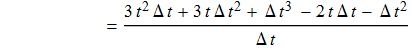
![]()

![]()
![]()
and,

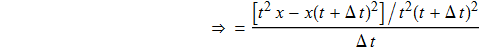

![]()
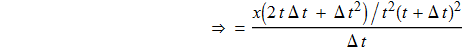
So,
![]()
![]()
![]()
![]()
![]()
![]()
![]()
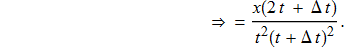
and

![]()
![]()
Choose one of the arguments by logic and prove it is true. A good project is to prove them all.
I have presented a fairly good reference for beginning to explore the mathematics used in physics. This is a good beginning.
[1] George E. Hrabovsky, (2009), Day 1: Introduction to Theoretical Physics. MASTers Notes, Issue 1, (http://www.madscitech.org/notes.html).
[2] Steven Galovich, (1989), Introduction to Mathematical Structures, Harcourt Brace Jovanovich. This truly wonderful book is out of print, but you can still find it here and there. It is my favorite book on logic, proofs, and set theory. I picked up my copy at a used book store for only $8.
[3] Joseph Fields, (?), A Gentle Introduction to the Art of Mathematics. This free textbook is available from the author's website: http://www.southernct.edu/~fields/GIAM/GIAM.pdf . This book goes much deeper than we intend to do.
[4] Michael A. Henning, (?), An Introduction to Logic and Proof Techniques. This is a free download from a course website: http://www.southernct.edu/~fields/GIAM/GIAM.pdf this set of notes is at about the right level for our purposes.
[5] Martin V. Day, (2009), An Introduction to Proofs and the Mathematical Vernacular. This is a free download from the website: http://www.math.vt.edu/people/day/ProofsBook. This book assumes that you have studied calculus.
[6] Dave Witte Morris, Joy Morris, (2009), Proofs and Concepts. This free book can be downloaded from the website: http://people.uleth.ca/~dave.morris/books/proofs+concepts.html. Sections I and II cover the topic of this writing.
Appendix: Arguments from Basic Mathematics
I am assuming that you will not need explanation for these. I include them for completeness and future reference.
In this section I will assume that you are familiar with the basic operations of arithmetic: addition, subtraction, multiplication, division, exponentiation, and root-taking. I will introduce a number of technical terms that will be understood without fomal definition.
| Argument | Name | Formula | Explanation |
| 82 | Fraction Multiplicaton | Multiplying fractions involves first multiplying the denominators and then the numerators. | |
| 83 | Fraction Division | Dividing fractions is just mutiplying the dividend by the inversion of the divisor. | |
| 84 | Cancellation | 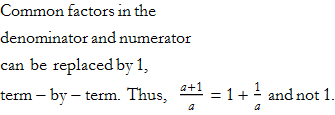 |
|
| 85 | Adding and SubtractingFractions | ||
| 86 | Adding Terms | n · a + m · a + b = (n + m) · a + b |
We can add like terms be adding their coefficients, unlike terms cannot be added. |
| 87 | Adding OppositeSignedIntegers | a + (-b) = a - b | Subtraction and adding opposite sign integers are equal. |
| 88 | AddingSame SignedIntegers | (-a) + (-b) = -(a + b) |
|
| 89 | Multiplying OppositeSignedIntegers | a · (-b) = -(a · b) | |
| 90 | Multiplying OppositeSignedIntegers | a · b = (-a)·(-b) | |
| 91 | DoubleNegative | -(-a) = a | |
| 92 | Multplying aTerm by 1 | We can always multiply a term by 1. | |
| 93 | MultiplyingExponents | ||
| 94 | DividingExponents | ||
| 95 | Reciprocal | ||
| 96 | Negative Power | ||
| 97 | Power of a Product | ||
| 98 | Power ofa Quotient | ||
| 99 | Rewriting Division | ||
| 100 | MultiplyingSame SignedIntegers | a · b = (-a)·(-b) | |
| 101 | Productof Roots | ||
| 102 | Quotient of Roots | 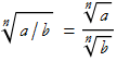 |
|
| 103 | Power of a Root | 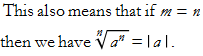 |
|
| 104 | Root as aFractional Power | ||
| 105 | The GeneralCommutativeProperty | a * b = b * a | Here we replace * by either + or ·. |
| 106 | The GeneralAssociative Property | (a*b) * c=a* (b * c) | Here we replace * by either + or ·. |
| 107 | DistributiveProperty | a · (b + c)=(a · b )+( a · c) | This is also the basis for factoring, in which case we reverse the process. |
| 108 | MultiplyingBinomials | (a + b)·(c + d) =(a · c) + (a · d) +(b · c) + (b · d) |
Proof of argument 82, Fraction Multiplication.
Assume that we have rational numbers x=a/b and y=c/d.
By the definition of a rational number, t/s, where s and t are integers, ![]() .
.
This is equivalent to the expression for integers (a÷b)·(c÷d).
We can rewrite this ![]() .
.
By the associative property of multiplication we can write this, ![]() .
.
By the definition of division we can rewrite this, (a·c)÷(b·d).
By the definition of rational numbers we have, ![]() .
.
Thus, ![]() , QED.
, QED.
This has been a direct proof.
In addition to logical operations. Mathematica is good at algebraic manipulations, too.
| Operation | Mathematica Command | Explanation |
| Simplify | Simplify[expr] | Performs a sequence ofsymbolic transformations on expr and outputs thesimplest form it can find. |
| FullSimplify | FullSimplify[expr] | Performs an extensivesequence of symbolic transformations on expr and outputs the simplest form it can find. |
| Expand | Expand[expr] | Expands all products andinteger powers for expr. |
| Factor | Factor[polynomial] | Factors a polynomial overthe set of integers. |
| Collect | Collect[expr,pat] | Collects terms of expr thatmatch pat. |
| Together | Together[rational] | Places the terms of a rational expression over a commondenominator and thencancels and factors in theresult. |
| Apart | Apart[rational] | Splits up a rationalexpression as a sum ofterms having minimal denominators. |
| Cancel | Cancel[rational] | Cancels common factors in a rational expression. |
| PowerExpand | PowerExpand[expr] | Expands all products andpowers for expr. |
First there are a few things to mention regarding Simplify. If we write,
![]()
![]()
you might think something went wrong. Why doesn't Mathematica return the correct value of x? This is because Mathematica doesn't know what number system we want to use. If we say that we want to consider only positive values of x then we write,
![]()
![]()
or even better still, if we say that x is an element of the set of real numbers, or symbolically x ∈ R,
![]()
![]()
this is the correct answer, the square root of ![]() in the reals is the absolute value of x.
in the reals is the absolute value of x.
Most of the time Simplify is good enough. For cases involving so-called special functions it is often best to use FullSimplify.
![]()
![]()
![]()
![]()
![]()
![]()
These are only a brief listing of the most basic capabilities of Mathematica in terms of algebraic manipulations. I invite you to explore the Documentation system and play with it.
Expanding on the ideas from the last section, we can define exponentiation and root-taking as inverse operations, similar to addition and subtraction. Thus we can define a root,
Definiiton 1: Root of an exponent: Given an exponent, ![]() , its nth root is a. This is denoted
, its nth root is a. This is denoted ![]() .
.
We can similary define the logarithm.
Definiiton 2: Logarithm of an exponent: Given an exponent, ![]() , its base-a logarithm is n. This is denoted
, its base-a logarithm is n. This is denoted ![]() .
.
| Argument | Name | Formula | Explanation |
| 109 | Logarithm of a product | The logarithm of a product isthe sum of the logarithms. | |
| 110 | Logarithm of a quotient | The logarithm of a quotient is the difference ofthe logarithms. | |
| 111 | Logarithm of a power |