George E. Hrabovsky
MAST
For the Chaos and Complex Systems Seminar Group. UW Madison, Department of Physics, 20 September 2016
The best model is based on a curve that we have perfect information about. People go to great lengths to assign curves to fit data. This leads to the belief that the curve so fitted corresponds to the behavior of the data and can predict the values of future data. Exact mathematical structures are the perfect basis of a perfect model.
So a model is an attempt to predict the future outcome of measurements. There are mathematical models that use the techniques of mathematics to make these predictions. There are computer models that use the techniques of computation to make such predictions. There are even physical models that are used.
The Marquis de Laplace once wrote, "We may regard the present state of the universe as the effect of its past and the cause of its future. An intellect which at a certain moment would know all forces that set nature in motion, and all positions of all items of which nature is composed, if this intellect were also vast enough to submit these data to analysis, it would embrace in a single formula the movements of the greatest bodies of the universe and those of the tiniest atom; for such an intellect nothing would be uncertain and the future just like the past would be present before its eyes."
This is the promise that modeling holds out to us.
The problem arises that nature rarely, if ever, truly corresponds to exact mathematical structures.
We thus need to approximate the structures in those cases where nature has chosen to be difficult.
The goal of a numerical model is to give an approximate, numerical, prediction of the behavior of a system.
If nothing changes then a system is boring. There is no point in making predictions for such a system.
Most things around us change over time. Mathematically,
a change in time can be written ![]() , or we could write
, or we could write ![]() , this is called a derivative operator. If we are looking at the change in temperature,
T, over time, we apply the operator to temperature
by writing
, this is called a derivative operator. If we are looking at the change in temperature,
T, over time, we apply the operator to temperature
by writing ![]() . If we apply this operator twice, then we
write
. If we apply this operator twice, then we
write ![]() , or
, or ![]() .
.
Unless you are using a computer algebra system, a programming language cannot calculate this directly. You either have to calculate it yourself and tell the language what the answer is, or resort to a numerical approximation method. If we equate a derivative to some quantity or set of quantities we have a differential equation. A simple such equation is a model for the behavior of an oscillator,
![]()
In Mathematica we can solve this directly and exactly.
We can get rid of the constants by establishing the initial position (denoted x[0]) and the initial velocity (denoted x’[0]).
Then we can display the output of the model for 10 seconds.
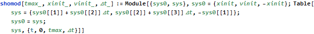
If we are not using Mathematica, or a similar system, we need to use a numerical scheme of some sort, here is how you do this in Mathematica.
This is called an Euler method and it is a way of breaking up the continuous flow of time encapsulated in the derivative into discrete chunks that the computer can handle. This is called discretization.
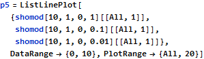
We can plot this for 10 seconds in units of one second.
This isn’t at all like the nice cosine curve we had above. We can either throw the model away, or we can try making the time steps more dense, say a tenth of a second.
This is a lot better, let’s try for a hundredth of a second.

We can combine these into a single plot.
We can compare this to the exact solution, with the blue curve being the exact solution..
Here we see the action of accumulating numerical error.
Note that we can have discretization of a region too. For example if we wanted to to see the propagation of temperature across a tabletop, we would need to discretize the tabletop. Just as with discretizing the time, discretization of spatial regions leads to accumulating errors, too
If there is error in measurement, there will be error in the models that represent such measurements. Related to this is the phenomena of coarse graining, which happens when phenomena are so close together that we do not realize there is any difference in them.
Every computer has a systemic error, called its machine error, or machine epsilon.
We have seen the result of discretization error.
Some numerical methods are better than others at getting close to an exact solution. In some systems we can choose a limit of accuracy and the system will keep making the intervals smaller until the desired accuracy is achieved. If a method is chosen that does not have this dynamic response, or the computer is unable to handle enough points to allow for the accuracy, then the method will not converge to the desired accuracy.
The error of each iterative step in time and in space is compounded.
Eventually the model will accumulate so much error that it looses all predictive capability.
Here we have the classical example of stability and instability: The Valley and the Hill.
Stable Point: Nearby trajectories point towards the fixed point
Unstable Point: Nearby trajectories point away from the fixed point. Each of these constitute a separate solution from the fixed point.
The behavior around the unstable point is called a bifurcation.
One iconic example of bifurcation is due to the logistic equation.
Before proceeding, we should state that when we have defined enough variables to gain complete information needed, we have established the state of the system.
If these variables change then we say that the state of the system changes, we have a change of state. Most models allow us to watch gradual changes of state. This occurs when some variable or parameter has changed. We have seen this in the oscillator model above, where the state (its position) changes with time.
There are situations where the change of state of a system occurs suddenly. Such as system is the Duffing oscillator. Here we see the amplitude of a Duffing oscillator with respect to its frequency.
This kinds of cycle that avoids a part of the trajectory is called hysteresis.
If you wish to delve more deeply into sudden changes in the state of a system, you can look into what is called catastrophe theory.
Chaos is another name for dynamic instability, that is instability that depends on the evolution of some variable or parameter, often time.
One check for this is the sensitivity of the behavior of a system to its initial conditions. There is a diagnostic for this sort of thing called the Lyapunov exponent. We can see an example of this in the logistic equation,
In physics we think of phase space as having axes of position and momentum. In mathematics it is a variable and its derivative. For the harmonic oscillator, the phase space looks like this.
pl10 = ParametricPlot[{Cos[t], -Sin[t]},
{t, 0, 10},
AxesLabel -> {x[t], p[t]}, BaseStyle ->
{Medium}]
![]()
Here is the phase space plot of the numerical approximation of the oscillator.
Here we see both of them at once.
For the Duffing oscillator we can plot the
first 100 time steps of its numerical solution
for three values within ![]() distance from each other.
distance from each other.
Here is the phase plot of the Duffing oscillator for the first 100 time steps. The blue strips represent the effects of varying the initial conditions by the small quantities specified above.
Laplace was wrong, even with perfect information you cannot predict the long-term behavior of a chaotic system. Here are some important concepts to take away with you:
Click here to go back to our home page.