The MAST Course on Relativity: Chapter Two

George E. Hrabovsky

MAST

Introduction

This chapter introduces several mathematical notions. I assume you have seen some set theory before this. If you are new to the ideas of set theory, I recommend Halmos’s excellent book called Naive Set Theory.

Manifolds

Last chapter we spoke of manifolds. We stated, almost as a definition, that manifolds were the arena where relativity lives. In point of fact, it is the place where any geometry occurs.

We can think of a manifold as some space having the local smoothness of Euclidean space, . Many authors use as it is the space of the set of n-tuples of real numbers, but it has a fixed origin. Since we need to speak of local frames of reference, we want to be able to establish new origins as we need them.

We don't really know what smoothness means, but maybe we can find out. How do we proceed without knowing what we mean? To understand this we will have to examine those properties of that produce local smoothness—whatever that is.

Recall that a set is a collection of all the elements of that set. If a set, U, is entirely a member of another set, M, then we say that U is a subset of M, we write this symbolically U⊂M. I do not propose that we delve into set theory, but it is the language used in mathematics so we will cover the bare necessities to proceed. The set of no elements is called the empty set, also called the null set, it is denoted Ø={}. The empty set is always a subset of any set. We can also establish a universe of discourse, or just the universal set, U, that contains every possible element we could ever be interested in. All sets are subsets of the universal set.

Recall that if we have two sets, A and B, we can establish a special set made up of the elements of both sets combined, called the union. This is written A∪B=(x|x∈A or x∈B}. We can also make a new set out of the elements that they have in common, called the intersection. This is written A∩B={x} x∈A and x∈B}. We can also create a new set by listing all elements of A that are not in B, this is called the difference and is denoted A-B={x}x∈A and x∉B}, where ∉ means not an element of ... . If we have the difference U-B, this is called the complement of B, this can also be written .

The set of points in a space is called, reasonably enough, a point set.

We can state that there is some rule, φ, that connects two sets, A and B, so that an element of A is converted into a unique element of B. Such a rule is called a mapping, or function. We then can write φ:A→B. A mapping where no two elements of A are mapped to the same point in B, is said to be one-to-one or equivalently injective. Such a mapping could be called an injection. We say that the image of φ is φ[A]={φ(x)}x∈A}.

A mapping from a subset of to is a fancy way of saying that you now have n functions of n real variables. If all of the partial derivatives of these n functions exist and are continuous, we say that such a mapping is or smooth. So now we know what smoothness means. To apply this idea to what we have already written about manifolds, it tells us that a manifold is some space whose local structure is represented by n functions of n variables whose partial derivatives exist and are continuous on . The spacetime manifold of chapter one is one such example of this.

Now we explore a little bit of topology. Let’s say that between any two points, say x and y, we can define the distance using the standard Euclidean distance in ,  d(x,y). A point set, O, that for every point, x∈O, a number ε>0 and that when d(x,y)<ε then y∈O, is called an open set. Simple examples of open sets are the open intervals of elementary calculus whose distance function is the absolute value.

To begin our hunt for what a manifold is, we begin by assuming that we have a set M.

We will also assume that we have a subset of M, U.

We will then establish a mapping .

We will state our first two rules,

C1: We will require that φ is injective.

C2: φ[U]=O is open, .

These structures can be combined, (U,φ), where we call such combinations n-charts or just charts. Another phrase used for a chart is a coordinate patch.

It seems that we might be able to use these charts to somehow make sure that our set M has this local smoothness structure we have been talking about. Why? Such a chart sets up a correspondence between the point set U⊂M and the open point set . In other words a chart defines n real-valued functions on U. These functions have all relevant partial derivatives and those are . Such a set of functions is what we call the smoothness structure. The points of U can be labeled by the values of these n functions. When charts overlap we will further require that they share the same smoothness structure. A collection of charts on a manifold is called an atlas. We will require that we are able to establish an atlas on M.

Above we introduced the notion of an injective mapping. We now state that a mapping μ:A→B where, for every element in B there is a unique element in A, we say that μ is onto or a surjection. A mapping that is both injective and surjective is called a one-to-one correspondence—or in less of a mouthful—bijection. Such a mapping is said to be bijective.

Say that we have two charts on M, (U,φ), and (U',φ'). If U and U' intersect in M, then their intersection, U∩U', will induce two smoothness structures on M. One smoothness structure comes from φ and defines a bijection between the intersection U∩U' and the image of that intersection in ,  . Another smoothness structure comes from φ' and looks a lot like the previous one; it defines a bijection between U∩U' and .

We can compose these mappings, .

We can also take its inverse .

Together these compositions form a bijection between φ[U∩U'] and φ'[U∩U']. It is this bijection that we can use to compare the smoothness structures of our proposed manifold. We now state two more rules:

Co1: φ[U∩U'] and φ'[U∩U'] are open subsets of .

Co2: The mappings and are .

If these conditions are met for a pair of charts, those charts are said to be compatible. For charts to be compatible we only require that they share the same smoothness property. In this way you can isolate a single smoothness structure. It is important to realize that (U,φ), and (U',φ') must be compatible if U and U' do not intersect.

We can have collections of sets, but we don’t want to call them sets of sets. Instead we call them families of sets. If we have a family of ten sets, each labeled M, we can index them using a subscript, . We can define a set i={1,2,…,10} and call this our index set. We can then define our family over the index set i by writing . As an example, we say that the third set of our family, according to our index set, is .

Let’s say we have a set, M, and we have a family of n-charts over an index set i on M, . If the following four conditions are met, then we call M an n-dimensional manifold.

M1: Any two charts of M are compatible. Another way of saying this is that if two charts induce a smoothness structure in the same region of M then those structures must agree.

M2: The charts cover M. This is another way of saying that all of M has an induced smoothness structure.

M3: Any n-chart compatible with the charts in the collection of charts C of M, is itself a member of C. This condition makes sure we are not overburdened with structure by limiting the number of charts we can put on M. By this condition we allow all compatible charts and remove all other structures.

M4: If we have distinct points in M, say p∈M and q∈M, then there will exist charts, and such that and where .

When we speak of manifolds, we write the label we have assigned and the charts are implied. There are different, but equivalent names for an n-dimensional manifold: -manifold (smooth manifold), Hausdorff manifold, and (this last is a mouthful) an n-dimensional manifold without boundary that is not necessarily paracompact or connected. In fact, the condition M4 prevents non-Hausdorff manifolds.

Given any set M with a set of n-charts C, such that C satisfies M1, M2, and M4, then M with C is a manifold.

Exercise 2.1: Show this last sentence to be true. If true we can always reduce the structure to that of a manifold by including more charts.

For example, say we have M as the set of n-tuples of real numbers. We can consider M a point set, so that we write . Let U be any subset of that is open. Let be the identity mapping. (U,φ) is a chart (check C1 and C2 to make sure). We see that this satisfies M1, M2, and M4, and that makes this a manifold. M3 is a lot harder to implement, but fortunately we do not need it.

As another example assume that M is the set of (n+1)-tuples of real numbers that also satisfy the equation . Define a point set having . Define the mapping as acting on the point , transforming to . Then we define another point set having . Define the next mapping acting on the point , this transforms to . Define a point set having . We define the next mapping that acts on the point , becoming . If we continue in this way we will find (2 n+2) charts, and , where i=1,2,…,(n+1). These n charts are all compatible. This produces an n-dimensional manifold called the n-Sphere, .

Exercise 2.2: Show that is indeed a manifold by this definition.

Assume we have two manifolds, M and N of dimensions m and n respectively. We can define a new manifold, P, called the product of M and N where we write, P=M×N. The dimensions of P will be m+n. P is a point set made up of the pair (p,q) where p∈M and q∈N. How do we introduce the required charts for this to be a manifold? Since M is a manifold we have a chart where and . Similarly for N, we have a chart where and . Since P=M×N, then we have the open subset . Now we need to establish our mapping. We use the points we defined above. We have which maps to . We also have which maps to . This leads us to map to , thus establishing . Thus we have . This gives us a chart on P, thus P is a manifold.

For example. we can take the product of the manifolds . We can see this as extending the 1-sphere, , along the set of real 1-tuples, . The resulting manifold is called the cylinder manifold.

Exercise 2.3: Draw a diagram of and satisfy yourself that it is a cylinder.

As another example, we can take the product of the manifold . Here we see that we are extending the 1-sphere, , along another 1-sphere, . The resulting manifold is called the torus manifold.

Exercise 2.4: Draw a diagram of and satisfy yourself that it is a torus.

We have previously defined an open set. We can extend this definition to cases where we have a chart. A set O is open in M if for any point p∈O, there is a chart (U,φ) where p∈U⊂O. A set is closed if its complement is open.

We can also construct new manifolds by cutting holes in existing manifolds, but only certain hole-cutting is allowed. Assume we have the manifold M and a subset of it, S⊂M. Here we state that S is open in M. Let C be closed and C⊂M. We now define N=M-C, with the charts (U,φ) on M where U∩C=Ø.

Exercise 2.5: Is N a manifold?

Before we move, let me say that for all of the fuss we have made about how to establish a manifold, they are completely boring objects. They are a blank canvas having a smoothness structure. They only become interesting when we put something on the canvas. Of course, linking back to our spacetime manifold this smoothness structure is what establishes the geometry of spacetime. If we make the assumption that spacetime is the world we live in, then the manifold contains the entirety of the dynamics of our world in its geometry.

Smooth Functions and Differentiable Mappings

Let’s say we have a manifold M, and we have some real-valued function, f, on M. If we have a chart on M, say (U,φ), then we can say that f:U→U, in other words f is a function from U to itself. We can state that is defined on .

Exercise 2.6: Why can we state this?

A less formal way of saying this is that is a real-valued function of n-variables.

Exercise 2.7: Let f be a function on M. Also let be for a collection of charts, C, satisfying M2 above. Show that f is a smooth function on M.

This is a standard technique for defining something on a manifold. You use a chart to describe that something in terms of . We will see why by the end of this chapter.

The collection of smooth functions on M is something that we will denote by the gothic F, F.

Exercise 2.8: Let be a function of m variables. Let represent a set of smooth functions on M, where the index set goes from 1 to m. Show that is a smooth function on M.

As stated in the last section, smooth functions on a manifold, M, characterize the manifold structure of M.

Let M be a set. let C and C' be two sets of charts on M satisfying M1-M4 from the previous section. If every smooth function on (M,C) is also a smooth function on (M,C'), then C=C'.

Exercise 2.9: Prove this last sentence to be true.

Exercise 2.10: Attempt to redefine a smooth mapping in terms of charts.

It is often the case in mathematics that when we introduce some class of objects that we also introduce some structure-preserving mappings between objects of the same class. Such structure-preserving mappings are called morphisms. We have mappings between sets, we have linear mappings (also called linear transformations) on vector spaces, and so on. The morphisms I want to present below are called differentiable mappings.

Let M and N be manifolds. Define the mapping μ:M→N. Assume there is a smooth function, f, on N. Then the composition f◦μ is a function on M.

Morphisms all share the property that a composition of morphisms is itself a morphism.

Theorem 2-1: Given the manifolds M, N, and O with smooth mappings and . Then the composition is also a smooth mapping.

Proof: Let g be a smooth function on O. We will show that the composition is a smooth function on M. Since g is a smooth function on O and is a smooth mapping, then is a smooth mapping on N. Since is a smooth function on N and is a smooth mapping, then is a smooth mapping on M. QED.

Two objects that are identical with regard to the definition of a structure being considered are called isomorphic. We say that two such objects share an isomorphism. We have already seen an example of isomorphisms of sets are what we have called bijections. Isomorphisms of vector spaces are simply called isomorphisms. Isomorphisms of manifolds are called diffeomorphisms. Let’s say we have two manifolds, M and N. Say that we have μ:M→N. If μ is bijective and is a smooth mapping, then we call μ a diffeomorphism. In such a case M and N are said to be diffeomorphic.

The composition of diffeomorphisms is a diffeomorphism.

Exercise 2.11: Prove this last sentence to be true.

Exercise 2.12: Prove that if two manifolds are diffeomorphic, they have the same number of dimensions.

Theorem 2-2: Let p∈M. There is an open set, O, containing p with the following property: given any point q∈O there will exist a diffeomorphism μ:M→M with μ(p)=q.

Proof: Let (U,φ) be a chart, and assume p∈U. Define . Now choose ε>0, such that and when d(x,z)<ε then x∈φ[U]).

The subset is our candidate for the open subset of M. Here V is the collection of all points with d(x,z)<ε.

Define a point q∈O such that where .

We can further make ε'=d(z,y)<ε.

We introduce the set [d(x,r)] and a function f(r) having the properties: NEEDS WORK

r1: f(r) is .

r2: There exists such that f(r)=1 when .

r3: There exists such that f(r)=0 when .

r4: .

We can see a prototypical example of this,

Exercise 2.13: Prove r1, r2, r3, and r4.

Since ε'<ε the function f(r) exists.

We now define a mapping, Λ:V→V such that,

This mapping is smooth by conditions r1 and r2. We can see by r2 that Λ(z)=y. By all four conditions we can see that Λ is the identity near the edge of V. We can also see that exists and is smooth.

Exercise 2.14: Show that the assertions of the previous paragraph are true. If necessary get hold of a book on Advanced Calculus and follow through a proof of the inverse function theorem and adapt it to this version of the theorem.

We can then define μ:M→M. If we say that s∈M we have two cases, s∈O or s∉O. If we accept the first case we write . If we accept the second case then we write μ(s)=s. It seems that μ is a smooth bijection, and that μ(p)=q. QED

Exercise 2.15: Prove that μ is a diffeomorphism.

This theorem seems to allow us to use charts to pull some specific property of into a property of the manifold M.

What we have done in this section is develop the ability to make connections from out manifold to archetypal sets that maintain the geometry of the manifold in the form of diffeomorphisms. This sets the stage for our ability to place things on our blank canvas.

Tangent Vectors in a Manifold

While in all generality we will be discussing geometrical objects throughout a manifold, it is convenient to begin by discussing objects at a point. To that end, let’s say we have a tangent vector located at a point, p, in denoted as . By establishing a local origin in we can treat it is if it were a local copy of , and this allows us to establish n-tuples—ordered sets of numbers having n elements, . We can thus write the n-tuple for the vector at the point, p, as . Each element of the vector n-tuple is a component of the vector in . In this way the vector can be represented by its components with respect to a set of coordinate axes (a chart) in , . Another way of saying this is that a tangent vector in is equivalent to a list of n real numbers. This is a completely natural representation of a vector in with a local origin. It is not necessarily so natural in an arbitrary manifold—where there need be no “natural” axes.

Assume that we are in . The collection of all smooth functions on will be denoted as . Thus an element of will be a real-valued function of n-variables, . Given a vector x having the set of components and also having a smooth function on , f, then we can define

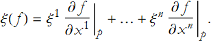
(2.1)

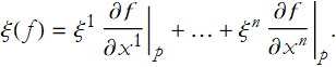
This is called a directional derivative of f in the direction represented by .

We can see from the elementary properties of derivatives that our directional derivative  ξ(f) will satisfy three conditions:

DD1: The Sum Rule: ξ(f+g)=ξ(f)+ξ(g)

DD2: The Power Rule: ξ(f g)=f(x)ξ(g)+g(x)ξ(f)

DD3: The Constant Function Rule: If f is a constant function, then ξ(f)=0.

We can see how this works with manifolds. Say we have our manifold, M. On this manifold we have a collection of smooth mappings, F(M). By Exercise 2.8, DD1, and DD2 we can see that the pointwise sum and product of elements of F(M) are also elements of F(M). For those of you who have studied abstract algebra this gives F(M) the structure of a ring.

Choosing a point, p, of M, then a tangent vector at p is a mapping , and this satisfies DD1, DD2, and DD3, where x is replaced by p. The collection of all tangent vectors in the manifold M located at p are denoted F(p). Our goal now is to show that F(p) is a vector space. To do that we begin by stating that ξ and η are in F(p). If we further state that we have some real number, say m, and an element of F, say f, then we can write (ξ + m η)(f)=ξ(f)+m η(f), and with this we are have accomplished our goal of establishing a vector space. We have shown how to add elements of the space and how to multiply elements by a real number.

Theorem 2-3: Equation 2.1 defines a bijection between the n-tuples and mappings from to . This bijection satisfies DD1, DD2, and DD3.

Proof: There are two things that we need to show to prove this theorem. The first is that equivalent directional derivatives have equivalent components. The second is that mappings from to satisfy DD1, DD2, and DD3.

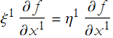To prove the first part let ξ(f)=η(f) for all f∈F. We set . Then by (2.1) we have . Since we can do this for all we have proved the first part.

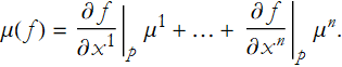
To prove the second part we state that there is a mapping, and that μ(f) satisfies DD1, DD2, and DD3. We can define a set of n values . This allows us to refine what we are trying to do. We now need to show that for this set of values (2.1) holds for all f. To accomplish this let , we we then rewrite f,

(2.2)

and where the set . To proceed we need to introduce a Lemma,

Lemma 2-4: If f is in then it can be written as (2.2) where p is some fixed point of for some .

Proof: We can write,

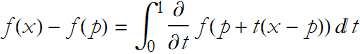
We can then write .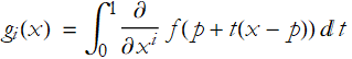

QED.

Continuing from this point, we apply DD! and DD2 to get

(2.3)

Since p is a fixed point we can use DD3 to state that μ(f(p))=0.

By using both DD1 and DD3 , so

By (2.2) , so

We can see that , so

This proves the second part. QED

Tangent vectors can also be represented in terms of charts. Given a chart on M, (U,φ), and where we label a smooth function f the composition is a smooth function on the image φ[U]. If our point p is in U, then we can write p=φ(p). We now introduce a set of n functions of F such that in an open subset of having our point p we get . In this way, if ξ is a tangent vector in our manifold at a point, then the set of numbers are called the components of the tangent vector with respect to the chart (U,φ).

Exercise 2.16: What is the purpose of the h functions?

Theorem 2-5: For a tangent vector, the choice of components is independent of the choice of h functions. In fact, given a set of components there exists a unique tangent vector in a manifold at a given point with those specific components.

Proof: Say that f is an element of the collection of smooth functions, F. If we also allow the functions , s, and t are also in F, such that s(p)=0. We can write f,

(2.4)

Exercise 2.17: Construct (2.4). Choose the set of functions so that on some open set containing p. Choose some s that is almost always positive, except that it vanishes at p. Choose t so that it satisfies (2.4).

Using an argument similar to that when we proved Theorem 2-3, and the fact that , we get

(2.5)

This proves our first statement, that the components are independent of the h functions.

The second statement of the theorem is proven by first noting that if we have a set of numbers , then 2.5 defines a tangent vector in M at the point p with the set of numbers as components. If M is an n-dimensional manifold, and p is a point in M, then the composition F◦(p) is an n-dimensional vector space.

The components of a vector depend on our choice of chart. We derive the well-known formula for this dependence. Let (U,φ) and (U',φ') be two charts, both containing the point p of M. Then U U' is handled in two ways, once by φ and once by φ’. That is to say we have a smooth bijection φ◦φ' from φ[U U'] to φ'[U U'], both subsets of . This gives us a set of n functions of n variables. We can write this set of functions, . Now let f be a smooth function on M. We can write and . If ξ is a tangent vector in M at p and and are it components with respect to our two charts (U,φ) and (U',φ') respectively. We can use (2.5) to conclude that

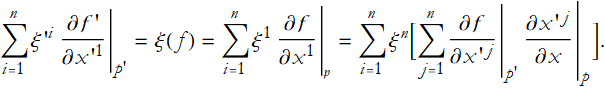
(2.6)

Since this must hold for all smooth functions,

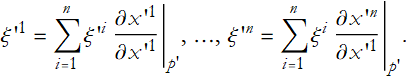
(2.7)

Doing this Stuff in Mathematica

While we can translate the formulas to perform calculations into Mathematica, most of the contents of this chapter are purely mathematical. In other words we are making mathematical definitions, and stating then proving conjectures. Mathematica has some theorem proving capabilities, but this requires listing all relevant axioms, definitions, and supporting theorems. This would require a book in itself, perhaps an interested reader will do such, alternately some crotchety old author might be convinced to add this to an ever-growing list of things to do. Here is an example of this kind of thing for group theory (some of which is now built-in to Mathematica). We begin by stating some group theory axioms (or gta) (establishing associativity, the identity, and the inverse—note that closure is implicitly understood).

We can now write a proof for the left-identity theorem.

So, somewhere in Mathematica is an 11 step proof of this theorem. We can now write it out in a nicely formatted form.

Doing this Stuff in Mathematica

While we can translate the formulas to perform calculations into Mathematica, most of the contents of this chapter are purely mathematical. In other words we are making mathematical definitions, and stating then proving conjectures. Mathematica has some theorem proving capabilities, but this requires listing all relevant axioms, definitions, and supporting theorems. This would require a book in itself, perhaps an interested reader will do such, alternately some crotchety old author might be convinced to add this to an ever-growing list of things to do. Here is an example of this kind of thing for group theory (some of which is now built-in to Mathematica). We begin by stating some group theory axioms (or gta) (establishing associativity, the right-identity, and the right-inverse—note that closure is implicitly understood).

We can now write a proof for the left-identity theorem. We begin by stating the cenjecture (by rights it shoyuld not be called a theorem until it is proved).

So, somewhere in Mathematica is an 11 step proof of this theorem. We can now write it out in a nicely formatted form.

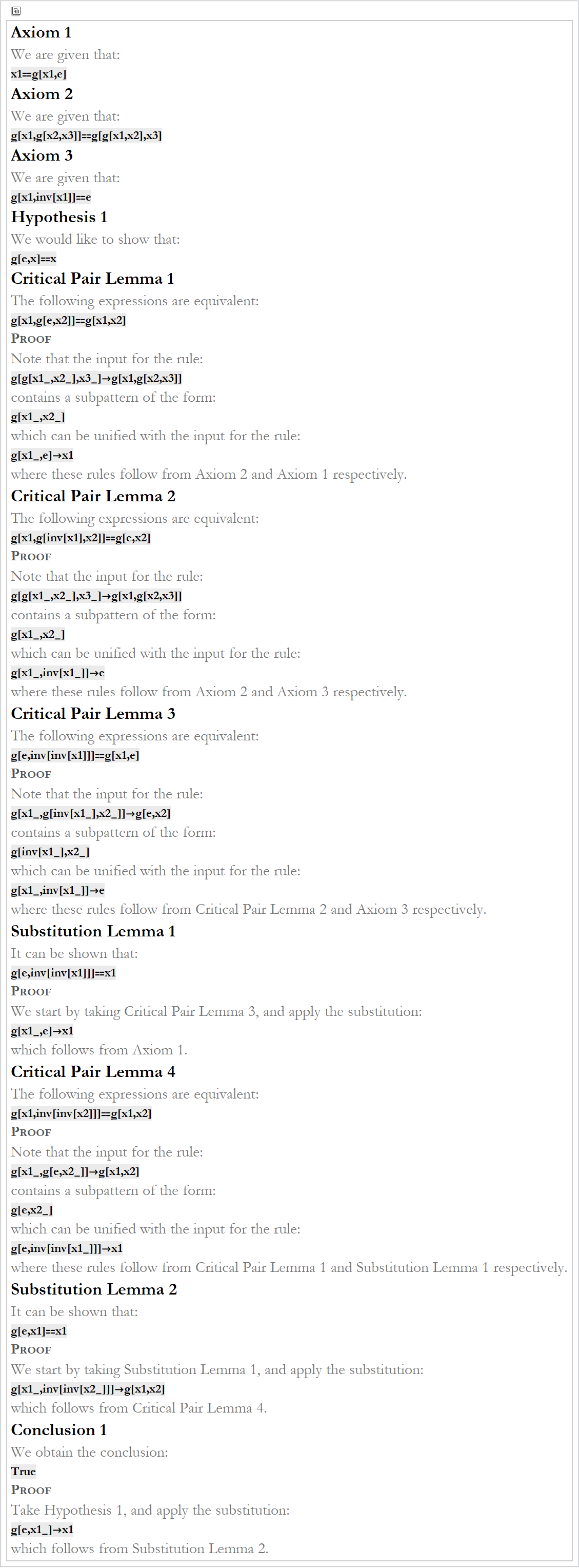
In the future we may add leftident to gta as we have proven it.

A systematic application of this would involve beginning with the rules of logic, then the rules of set theory, then advanced calculus, and then abstract algebra.  Then you could proceed step-by-step to prove each theorem in differential geometry by listing any new axioms and including all proven statements as new statements to be used in proofs.