The MAST Course on Relativity: Chapter One
George E. Hrabovsky
MAST
The Magic of the Speed of Light
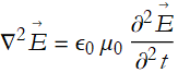
Were we to begin with the electromagnetic wave equations we would be able to derive the Laplacian of the electric field for a place having no charge or current,
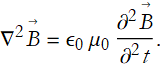
and we find the same combination of weird symbols, ![]() , in the Laplacian of the magnetic field
, in the Laplacian of the magnetic field
It turns out that if we examine the ability of magnetic fields to pass through a vacuum, we encounter a number ![]() , this is the quantity called the magnetic permeability, it has been given one of the symbols encountered above,
, this is the quantity called the magnetic permeability, it has been given one of the symbols encountered above, ![]() . There is also the quantity representing the ability for the electric field to pass through the vacuum, this is approximately
. There is also the quantity representing the ability for the electric field to pass through the vacuum, this is approximately 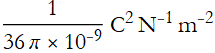 and is called the permittivity of space; and is given the other symbol from above,
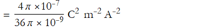
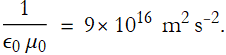
 ![]() . If we multiply them we have
. If we multiply them we have
![]()
![]()
![]()
The Ampere can be written as C/s
![]()
![]()
We then invert this product,
Strangely enough this has units of speed squared. This makes sense since the coefficient of the second-order time derivative in the Laplacian should be the inverse wave propagation speed squared. Now, here is a remarkable thing, if we take the square root of this,
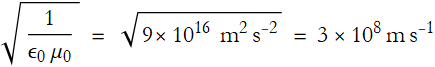
and we look at the right-hand result long enough we will realize that this is approximately the speed of light in a vacuum! To put it another way, the square root of the inverse product between the ability of empty space to allow electric and magnetic fields to propagate is the speed of light in empty space. Looking at the Laplacian this tells us that the speed of light is the speed of an electromagnetic wave in empty space. This tells us that electricity, magnetism, and light are all aspects of the same thing.
Since the speed of light in a vacuum is determined by the use of fundamental constants, then it seems reasonable to postulate that the speed of light in a vacuum is itself a constant. The value of  was first measured by Wilhelm Eduard Weber and Rudolf Kohlrausch in 1856. The discussion of the Laplacians is due to James Clerk Maxwell.
This seems almost circular today since we now determine the values of ![]() and
and ![]() in terms of the speed of light.
in terms of the speed of light.
The Postulates of Special Relativity
Einstein formulated two postulates when he derived the special theory of relativity:
Postulate 1: The laws of physics are the same in any inertial frame of reference.
This is just the principle of relativity due to Galileo. I am assuming that you know what a frame of reference is.
Postulate 2: The speed of light is a constant, and nothing can move faster than the speed of light in empty space.
We just made a strong argument for the truth of the assumption of the constancy of light speed. It makes sense to say that nothing can move faster than the speed of information transfer (or else you could have the situation that the effect of an action could be seen to precede its cause). We can easily infer that the speed of information transfer is that of light.
Let the weirdness follow.
Natural Units
The first ramification of Postulate 2 is the ability to avoid having to write out the speed of light in SI units every time we need to do a calculation. The speed of light can be approximated as ![]() to make it easier to write in SI. This is still unwieldy.
to make it easier to write in SI. This is still unwieldy.
Now, we have to realize that SI units are not natural units. Nature did not assign the meter or the second as fundamental. We can choose whatever units we want so long as they are consistent. We can choose our unit of time to be the time it takes light to travel one meter and call this unit a meter of time.
The speed of light is then,

So, the speed of light is 1. This may seem startling, but it is a very natural way of looking at it. In fact, that is the name for this system of units, they are called natural units. There are other units in this system, but we will not concern ourselves with them for now.
Special Relativity, Events, and Spacetime
Let’s say you want to describe a physical system. We first need to understand and establish the space of states that the system can find itself in. At any given time the system will be found in one such state. As the system experiences the passage of time you will find that the system evolves through a sequence of states. Such a system is called a dynamical system.
Any occurrence in the physical world is called an event. Events have no extent in either space nor time. As such they can be represented by a point.
The set of all events that will happen, have happened, and are happening is what we mean by spacetime. We can denote this spacetime by the label M. In this way an event in spacetime is sometimes called a point in M. Here, of course, M is the state space in relativity.
We use a neat device for studying space and time in relativity, it is called a spacetime diagram. It looks similar to a normal coordinate frame except the time axis is vertical and the spatial axes are perpendicular to it and each other (for three spatial dimensions this becomes impossible to visualize).
To identify the location of an event in spacetime we need four coordinates. We can write these ![]() ,
, ![]() ,
,![]() , and
, and ![]() . We can also write this as
. We can also write this as ![]() where we understand that μ is allowed to be summed from 0 to 3. If we restrict such coordinate systems to be in uniform linear motion, we say that that coordinate system is an inertial frame. An inertial frame is sometimes also called an inertial reference frame or inertial reference system. Each observer in uniform linear motion is at the origin of their own reference frame within a region of spacetime, thus we can call them inertial observers.
where we understand that μ is allowed to be summed from 0 to 3. If we restrict such coordinate systems to be in uniform linear motion, we say that that coordinate system is an inertial frame. An inertial frame is sometimes also called an inertial reference frame or inertial reference system. Each observer in uniform linear motion is at the origin of their own reference frame within a region of spacetime, thus we can call them inertial observers.
A single point in spacetime, P, is what we have called an event. In a spacetime diagram we have,
Say that we have two inertial frames in the same region of M. Let's say that we label one system as ![]() and the other as
and the other as ![]() . For each such system we can measure every event in M. Since we can observe the same event on different spacetime diagrams, we should be able to use that event to place one spacetime diagram into another by drawing the relative coordinate axes. We can represent this on a spacetime diagram, assuming that the
. For each such system we can measure every event in M. Since we can observe the same event on different spacetime diagrams, we should be able to use that event to place one spacetime diagram into another by drawing the relative coordinate axes. We can represent this on a spacetime diagram, assuming that the ![]() system is moving with some velocity v with respect to the
system is moving with some velocity v with respect to the ![]() system. In a spacetime diagram the
system. In a spacetime diagram the ![]() axis is the locus of constant
axis is the locus of constant ![]() . Since
. Since ![]() is moving at some velocity v, this axis will not longer be vertical, but will be tilted in the
is moving at some velocity v, this axis will not longer be vertical, but will be tilted in the ![]() direction.
direction.
In order for the ![]() system to look at the event located at P at some time
system to look at the event located at P at some time ![]() , we must shine a light on it. This light originates from a point
, we must shine a light on it. This light originates from a point ![]() .
.
Since the y system determines the coordinates of an event, as does the x system, we can write the y coordinates as functions of the x coordinates, ![]() ,
, ![]() ,
, ![]() , and
, and ![]() . Clearly we cannot use the same general index for both x and y. We can use μ for x,
. Clearly we cannot use the same general index for both x and y. We can use μ for x, ![]() , and ν for y,
, and ν for y, ![]() . Thus we have
. Thus we have ![]() . It is reasonable to assume that such a function is smooth,
. It is reasonable to assume that such a function is smooth, ![]() , if we are careful in our choice of coordinates. If the y values are smooth functions of the x coordinates, then the inverse functions should also be smooth and we can write,
, if we are careful in our choice of coordinates. If the y values are smooth functions of the x coordinates, then the inverse functions should also be smooth and we can write, ![]() .
.
Exercise 1.1: Show this last sentence to be true.
From this we can see that we have the possibility of a large number of coordinate systems, any two of which can be smoothly related to one another. This leads us to the notion of a specific mathematical object, a four-dimensional manifold. It is important to understand that such an application of mathematical structure can never be proven in a rigorous way, it can only ever be assumed. There is never any guarantee that such a choice of structure will gain any advantage. Once it is made, though, we need to stick with it—that is how a theory is developed. We will be certain to assume that all statements about physical phenomena in spacetime will be considered about points in the spacetime manifold M.
If we allow an event to take some small time over a small distance to occur, ![]() , called the spacetime interval. If we then choose units of distance and time so that the speed of light c does not change, we then write
, called the spacetime interval. If we then choose units of distance and time so that the speed of light c does not change, we then write
![]()
(1.1)
and we say that the spacetime interval of an event is invariant. No matter what your inertial frame, the spacetime interval between events will be the same. Space and time will distort to make sure this interval is invariant.
Let’s say that we are watching a particle move through M. Were we to follow the motion of this particle through its evolution of states in spacetime, we would see it evolve into a smooth curve. We call such a curve a world line. A world line completely defines the past, present, and future of a particle for its existence.
We can extend this to higher dimensional objects. If we follow a string it evolves into a world sheet. Similarly a membrane would sweep out a world volume. Particles that collide would have their world lines intersect where the point of intersection is the location of the event of their collision.
The important thing to realize is that in this view of spacetime nothing ever really happens, it is already laid out in its future, present, and past. There is no dynamics, it is all geometry.
There is an illusion of motion in spacetime. This illusion occurs when we consider a stack of spatial surfaces where each surface is encoded with a specific time parameter. As we allow time to evolve from one surface to the next, world lines are traced out in spacetime.
Thus we can recover dynamics by slicing spacetime into a stack of three-dimensional surfaces. There is no natural process of slicing spacetime with these surfaces. Since these are surfaces of constant time, isochronous surfaces, there can be no natural concept of simultaneity. We will see that this mechanism leads the way to numerical relativity.
Tangent Vectors, One-Forms, and Tensors
Any set of four quantities ![]() that transform under a change of coordinates in the same way as the spacetime interval
that transform under a change of coordinates in the same way as the spacetime interval ![]() according to (1.1) form what is called a tangent vector, sometimes called a contravariant vector, since the transformation of basis vectors produces an inverse transformation in components. The invariant quantity
according to (1.1) form what is called a tangent vector, sometimes called a contravariant vector, since the transformation of basis vectors produces an inverse transformation in components. The invariant quantity
![]()
(1.2)
may be called the squared norm of the tangent vector. With a second tangent vector ![]() , we have the scalar product invariant
, we have the scalar product invariant
![]()
(1.3)
In order to get a convenient way of writing such invariants we introduce the technique of lowering indices. Define
![]()
(1.4)
Then the expression on the left-hand side of (1.2) may be written ![]() , it is understood that a summation is to be taken over the four values of μ. It is important to note that
, it is understood that a summation is to be taken over the four values of μ. It is important to note that ![]() is a scalar, the indices vanish and we are left with the scalar product invariant of A and A. With the same notation we can write (1.3) as either
is a scalar, the indices vanish and we are left with the scalar product invariant of A and A. With the same notation we can write (1.3) as either ![]() or else
or else ![]() . Here we are also left with a scalar, we say that the indices are contracted. The scalar product invariant (A,B) remains.
. Here we are also left with a scalar, we say that the indices are contracted. The scalar product invariant (A,B) remains.
The four quantities ![]() introduced by (1.4) may also be considered as the components of a geometrical object similar to a vector. Their transformation laws under a change of coordinates are somewhat different from those of the
introduced by (1.4) may also be considered as the components of a geometrical object similar to a vector. Their transformation laws under a change of coordinates are somewhat different from those of the ![]() , because of the differences in sign, and the object is called a one-form (or in some literature, a covector, or a covariant vector since when we transform the basis vectors the components transform in the same way).
, because of the differences in sign, and the object is called a one-form (or in some literature, a covector, or a covariant vector since when we transform the basis vectors the components transform in the same way).
From the two tangent vectors ![]() and
and ![]() we may form the sixteen quantities
we may form the sixteen quantities ![]() . These sixteen quantities form the components of a tensor of the second rank. This is sometimes called the outer product of the vectors
. These sixteen quantities form the components of a tensor of the second rank. This is sometimes called the outer product of the vectors ![]() and
and ![]() , as distinct from the scalar product (1.3), which is also called the inner product. The outer product is sometimes called the tensor product and is denoted
, as distinct from the scalar product (1.3), which is also called the inner product. The outer product is sometimes called the tensor product and is denoted ![]() .
.
The tensor ![]() is a rather special tensor because there are special relations between its components. But we can add together several tensors constructed in this way to get a general tensor of the second rank,
is a rather special tensor because there are special relations between its components. But we can add together several tensors constructed in this way to get a general tensor of the second rank,
![]()
(1.5)
The important thing about the general tensor is that under a transformation of coordinates its components transform in the same way as the quantities ![]() .
.
We may lower one of the indices in ![]() by applying the lowering process we used above on each of the terms on the right-hand side of each expression in (1.4). Thus we may form
by applying the lowering process we used above on each of the terms on the right-hand side of each expression in (1.4). Thus we may form ![]() or
or ![]() . We may lower both indices to get
. We may lower both indices to get ![]() .
.
Exercise 1.3: What happens when we lower the indices of ![]() to get either
to get either ![]() ,
, ![]() , or
, or ![]() ?
?
In ![]() we may set ν=μ and get
we may set ν=μ and get ![]() . We will always sum over the four values of μ when an index appears twice in a term . Thus
. We will always sum over the four values of μ when an index appears twice in a term . Thus ![]() is a scalar.
is a scalar.
Exercise 1.4: Show that ![]() is a scalar C.
is a scalar C.
It is equal to ![]() .
.
We may continue this process and multiply more than two vectors together, taking care that their indices are all different. In this way we can construct tensors of higher rank. If the vectors are all contravariant, we get a tensor with all its indices as superscripts. We may then lower any of the indices and so get a general tensor with any number of indices superscripts and/or subscripts.
We may set a covariant index equal to a contravariant index. We then have to sum over all values of this index. The index becomes a dummy index. We are left with a tensor having two fewer effective indices than the original one. We saw this above for vectors, this process for tensors is also called contraction. Thus, if we start with the fourth-rank tensor ![]() , one way of contracting it is to put σ = ρ, this gives the second rank tensor
, one way of contracting it is to put σ = ρ, this gives the second rank tensor ![]() having only sixteen components, arising from the four values of μ and ν. We could contract again to get the scalar
having only sixteen components, arising from the four values of μ and ν. We could contract again to get the scalar ![]() .
.
We can now appreciate the balancing of indices. Any effective index occurring in an equation appears once and only once in each term of the equation, and always contravariant or always covariant. An index occurring twice in a term is a dummy, and it must occur once contravariant and once covariant. It may be replaced by any other Greek letter not already mentioned in the term. Thus ![]() . An index must never occur more than twice in a term.
. An index must never occur more than twice in a term.
Enough mathematical formalism for now. Let’s get back to physics.
Lorentz Transformations
Getting back to our example from above, we see that the light beam forms a world line that crosses the ![]() axis at the point
axis at the point ![]() .
.
Once the light beam reflects off the event P it returns to the ![]() axis.
axis.
The reflected light beam crosses the ![]() worldline at
worldline at ![]() .
.
If we assume that the light beam leaves at time ![]() and is reflected back at
and is reflected back at ![]() we can fix the coordinates of our event,
we can fix the coordinates of our event,
We can make this more useful by stating that the initial time occurs at some unit T, ![]() , the event P itself occurs at some factor of the initial time later,
, the event P itself occurs at some factor of the initial time later, ![]() , and
, and ![]() . We now have
. We now have
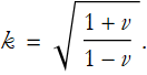
Recall from elementary kinematics,

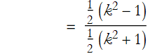
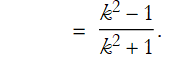
We can solve this for k in terms of v,
We can see that ![]() will occur a factor, k, later than
will occur a factor, k, later than ![]() , so
, so
![]()
and similarly,
![]()
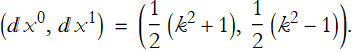
If we solve this system of equations we get,
(1.6)
and
(1.7)
These are the famous Lorentz transformations, and they tell us how to look at one coordinate system from another. If we make the definition

(1.8)
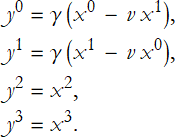
The Lorentz transformations then become,
![]()
![]()
![]()
![]()
(1.9)
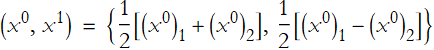
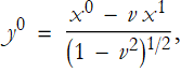
From this we see that, ![]() if and only if
if and only if
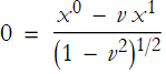
![]()
![]()
Thus we have the ordered pair ![]() for the
for the ![]() coordinate.
coordinate.
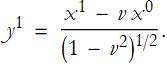
Similarly, ![]() if and only if
if and only if
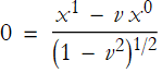
![]()
![]()
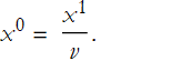
This gives us the ordered pair 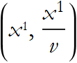 for the spatial
 ![]() coordinate.
coordinate.
We see that the spacetime diagram now looks something like this,
This is called a boost in the ![]() plane. There is a change in velocity, but no rotation. The collection of all boosts and all spatial rotations form the Lorentz group, but we will not go into the details here. The group of transformations satisfying the equation,
plane. There is a change in velocity, but no rotation. The collection of all boosts and all spatial rotations form the Lorentz group, but we will not go into the details here. The group of transformations satisfying the equation,
![]()
(1.10)
is called the Poincaré group. Thus the Poincaré transformations consist of the Lorentz transformations followed by a spacetime translation.
The Light-Cone Structure
Nothing moves faster than light. This is one of the assumed facts of special relativity. We can use it to examine yet another piece of the structure of a spacetime manifold.
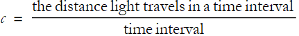
Faster implies speed. Speed is defined as distance traveled—displacement—per unit of time. This idea is fundamentally incompatible with the idea of spacetime.
Exercise 1.5: Explain this incompatibility.
So the idea of moving faster than anything requires a reformulation in order to fit into the concept of spacetime. Suppose that an event occurs in spacetime, at which point a spherical pulse of light is emitted. No particle whose world line passes through this point in spacetime (the event) can ever escape from the spherical pulse. In this way we can say that the particle cannot exceed the speed of light. Were we to label the event p then we can represent the expanding pulse as a cone in spacetime whose vertex is located at p. We can see in such a case that the world line of the particle passing through the event p lies inside the cone.
From this we can see that there is, for every event in M a cone whose vertex is that event. The world line of a particle that passes through the vertex event lie inside the cone. We will call such a cone a future light cone.
Say that we have two future light cones that are close to each other in spacetime. If an event q lies inside the future light cone of the event p, then we say that q is timelike with respect to p. In this case we say that q lies in the future of p.
If p lies in the future of q, then we say that q is timelike related to p and is in its past.
If q lies on the future light cone (or the past light cone) of p we say that q is null related to p in the future (or the past).
If neither event is within nor on the light cone of the other, then we say that the events are spacelike related to the other.
In flat spacetime, special relativity, you can arrange things so that all light cones look like normal cones—they all have the same opening angle and the timelike axes are all parallel. There is no reason to make such an assumption in a generic way. In general relativity, where we admit curved spacetime, this assumption is no longer justifiable. Indeed, avoiding this assumption is equivalent to assuming such curvature.
Four-Scalars
Thus far, for the sake of simplicity, we have been considering spacetime as having only one spatial dimension. Of course, we know that in the real world there are three apparent spatial dimensions. This gives us a total of four dimensions, so the spacetime interval is,
![]()
Adopting the convention that a Latin index is summed from 1 to 3, we can rewrite this
![]()
(1.11)
This is a four-dimensional quantity that is invariant. Such a quantity is called a four-scalar.
Four-Vectors and Index Gymnastics
We can consider the four-dimensional Lorentz transformations
(1.12)
We can make a 4 4 matrix of the coefficients for the system of equations in (1.12),
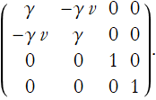
(1.13)
We can name this matrix ![]() and name it the metric tensor.
and name it the metric tensor.
We can make a transformation to a new set of coordinate axes, where each of the ![]() of (1.1) becomes a linear function of
of (1.1) becomes a linear function of ![]() of the new set of axes so that the quadratic form (1.1) is a general quadratic form,
of the new set of axes so that the quadratic form (1.1) is a general quadratic form,
![]()
(1.14)
where ![]() .
.
If we have a four-dimensional vector that undergoes a Lorentz transformation, we call it a four-vector. A generic four-vector, ![]() , has the form
, has the form
![]()
(1.15)
Let’s say we have another four-vector, ![]() . We can then can define another four vector as the linear combination
. We can then can define another four vector as the linear combination ![]() when λ is given a value. Its squared length is
when λ is given a value. Its squared length is
![]()

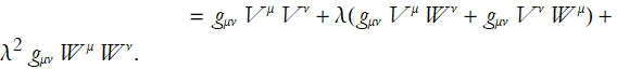
(1.16)
This must be an invariant (four-scalar) for all values of λ. It then follows that each term is separately an invariant.
The coefficients of λ are then
![]()
(1.17)
we can interchange the indices in the second term,
![]()
(1.18)
so that we can rewrite (1.17)
![]()
(1.19)
From this we see that the second term in (1.16) is an invariant, it is the inner product of ![]() and
and ![]() .
.
We can define g as the determinant of ![]() . If this determinant were to vanish (g=0), then the four axes would not provide independent directions in spacetime. We thus assert that the determinant must not vanish. If we have orthogonal axes, the diagonal elements of
. If this determinant were to vanish (g=0), then the four axes would not provide independent directions in spacetime. We thus assert that the determinant must not vanish. If we have orthogonal axes, the diagonal elements of ![]() become 1, -1, -1, -1 and the off-diagonal elements are all 0. From this we can calculate g=-1.
become 1, -1, -1, -1 and the off-diagonal elements are all 0. From this we can calculate g=-1.
Exercise 1.6: Perform this calculation.
For oblique axes, similar to those given by a Lorentz transformation, g must still be negative.
Exercise 1.7: Why is this true?
We now define a one-form ![]() such that,
such that,
![]()
(1.20)
Since g≠0, we can solve these equations for ![]() ,
,
![]()
(1.21)
We calculate each ![]() as the cofactor of the corresponding
as the cofactor of the corresponding ![]() in its corresponding determinant, divided by the determinant itself.
in its corresponding determinant, divided by the determinant itself.
If we substitute the value of ![]() from (1.20) with that in (1.21)
from (1.20) with that in (1.21)
![]()
(1.22)
This equation must be true for any four quantities ![]() we can make the inference,
we can make the inference,
![]()
(1.23)
where ![]() is the Kronecker delta.
is the Kronecker delta.
We can use (1.20) to lower any index in a tensor. We can use (1.21) to raise any index in a tensor. Raising and lowering indices are operations that are collectively called index gymnastics. These rules are all applications of contraction.
Doing this Stuff in Mathematica
I will now reproduce significant results in Mathematica. Where we use tensors and other indexed objects I will use the free package xAct.
We will start by duplicating our first calculation above. Mathematica allows us to incorporate units into our calculations.
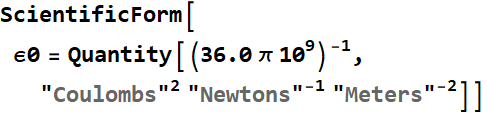
![]()
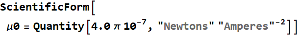
![]()
![]()
![]()
Here we apply the unit conversion for the Ampere,
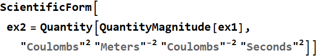
![]()
Note that Mathematica does not evaluate the units correctly. We can apply the unit conversions for the Ampere by hand and include the units ![]()
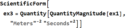
![]()
Then we invert this,
![]()
Ten we take the square root,
![]()
![]()
which is approximately the speed of light.
For the tensor analysis portion we will need to load xAct.
![]()

![]()

![]()
![]()

![]()


We next need to establish our spacetime manifold. We will use the DefManifold command:
DefManifold[M, dim, {a, b, c, ...}] defines M to be the label we will use for an dim - dimensional differentiable manifold. This label can be anything we want it to be. We then write dim as the number of dimensions in the manifold. This can be a positive integer, or it can be a constant symbol. Then we list the abstract indices a, b, c, ... that will be used by our tensors. In our case we will define a manifold called M4, it will have four dimensions, and it will use a number of lower - case Greek letters. I will use the Greek letters, because most symbols I will want to use will not interfere with the chosen indices.
![]()
![]()
![]()
We can define a tangent vector,
![]()
![]()
![]()
| tv |
|
We can define a one-form,
![]()
![]()
![]()
| of |
|
We can define a general tensor
![]()
![]()
![]()
| Ct |
|
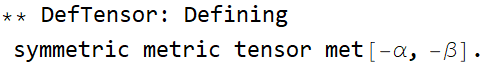
We can define the metric tensor,
DefMetric[sign of the determinant, the label of the metric and its indices, the label for the covariant derivative, {the symbols associated to the covariant derivative}, and how to print the metric]
![]()

![]()

![]()
![]()
![]()
![]()
We can demonstrate (1.23).
![]()
| δ |
|
we can demonstrate metric contraction.
![]()
| Ct |
|
![]()
| Ct |
|