Chapter Two: Functions
Sets and Functions
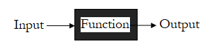
What is a function? One possible answer is that it is a machine, or a black box, that takes a value as input and it gives you some output in return (see Fig. 2.1).
Figure 2.1. A Function as a Black Box Machine.
But that tells us nothing about what a function actually is, it simply describes what a function does. Any definition that describes something’s behavior instead of its fundamental nature is called an operational definition. Sometimes an operational definition is all we can provide until we know more.
Let’s explore this idea in more detail. If a function can be thought of as a mechanism for transforming some input into some output, then it must have the means for producing the output from the input. There must be some rule, either simple or complicated, that decides how the output is generated from the input. So the function must be that rule. Thus we can say that a function is a rule that takes some input value and converts it into an output value. In this way we can see that a function is sometimes called a transformation.
If the input value is allowed to be any element of a given set, then we can call the input the independent variable. We can, similarly, call the output the dependent variable, since its value is dependent upon the input. If we call the input x and the output y, we can say that y is a function of x. Symbolically we can assign the symbol f to the rule of the function. We can, of course, use any symbol we like to represent the function so long as we are consistent about it
We can write the application of the rule to the input as the symbol f(x). So the sentence above is often written in symbols,
![]()
(2.1)
While often written this way due to tradition, it is more correct to use the notation |→ to signify that the symbol to the left of the arrow turns into the symbol to the right. So (2.1) becomes,
![]()
(2.2)
this is also written
![]()
(2.3)
and we would say, “the value ofy is the operation of the function f on the value of x.”
Apprentice Exercise 2-1: If we can write the rule of the function to be f(x)=x+1, then the function can be written abstractly as f□=□+1 where we replace □ by the independent variable. For the following functions identify the rule.
a) ![]()
b) 
c) ![]() .
.
To understand functions in more depth we must examine some language of mathematics. We begin by saying that we can collect some related things if they follow three rules that we will assume to be true, we will call such assumptions by the name axioms, or equivalently, postulates. The first rule is that if x is a given mathematical object under study, it is either part of our assembly or it is not. This tells us that for any such collection there is some rule defining what constitutes a member of the collection. We will call this rule S1. The second rule is that each member of a collection must be distinguishable from all other members, thus we only note a given member once. We will call this rule S2. The third rule is that no collection can be a member of its self. This rule is called S3. Any collection for which S1, S2, and S3 hold true is called a set.
Journeyman Exercise 2-1: What problems can we run into if we remove either S1, S2, or S3 from the definition of a set?
If the object x is a member of the set X we will write
![]()
(2.4)
if x is not an element of the set X, we write,
![]()
(2.5)
A set that has no elements is called either the empty set, or the null set. It is written Ø.
While no set can be an element of itself, if all elements of the set A are also elements of the set B, we say that A is a subset of the set B. We write this using the symbol ⊆. So,
![]()
(2.6)
Two sets are said to be equal if they are each subsets of each other. In shorthand we use the symbol ∧ for the word and, and we also use the symbol ⇒ for the word if or implies. For equality we write,
![]()
(2.7)
Apprentice Exercise 2-2: Translate (2.7) into its English equivalent.
If A is a subset of B and A is not equal to B, A is a proper subset of B. We write this,
![]()
(2.8)
We can now show the set theory definition of a function, often called a mapping. Such a function maps every element of the set A to a unique element of the set B. This is written with the symbol representing the phrase, “for every,” or, “for all,” with ∀, and the symbol for the phrase, “there exists,” with ∃. We write the sentence defining a mapping,
![]()
(2.9)
Apprentice Exercise 2-3: Translate (2.9) into its English equivalent.
The function f maps the set A to the set B. The act of mapping is denoted by the long arrow →. We write
![]()
(2.10)
We can also make a diagram (see Fig 2.2).
![]()
Figure 2.2. The Function as a Mapping from one set to another.
The set from which all independent variables are drawn is called the domain. The domain for the mapping from (2.10) or (Fig. 2.2) is the set A and is denoted D(f). The independent variables are the elements of the domain. The set from which all dependent variables are drawn is called the codomain, and is the set B. The specific dependent variables form a new set called the range, R(f). and this is a subset of B. The range need not be the entire codomain.
Any connection between ideas, or equivalently any connection between symbols is called a relation. We are being a bit sloppy in our terms. Let’s try to be more precise. Let’s say that we have a pair of sets A and B. Then we have something that links at least some elements of A to some elements of B. Assuming that a describes some element or elements of A and b some element or elements of B, the relation that links the elements is generically symbolized by R, so we write a R b.
There are many ways to combine sets, and we need to combine them in a special way. Before we get to that way we should examine some simple combinations that you might be familiar with. If we list all elements of two sets as if it were one set, applying S1 through S3, then we get a set that is called the union of the two component sets, and we symbolize the union ∪. In fact if the two sets are our objects, we can treat the union symbol as the relation. If we say that the sets are A and B, then we write A ∪ B, where the ∪ symbol is the relation between the sets. We can write this formally, if we use the symbols | for the phrase, “such that”, and ∨ for the word or,
![]()
(2.11)
Apprentice Exercise 2-4: Translate (2.11) into its English equivalent.
Another way to produce a new set from two existing sets is to list all of the elements that the two sets have in common. We call the new set the intersection of the component sets and use the symbol ∩. The relation in this case is written A∩B. This is written formally,
![]()
(2.12)
Apprentice Exercise 2-5: Translate (2.12) into its English equivalent.
We can also write a new set as the elements of one set that are not elements of the second set. This is called the difference and is symbolized with \. So the relation will be written A \ B. We can write this formally,
![]()
(2.13)
Apprentice Exercise 2-6: Translate (2.13) into its English equivalent.
Now we get to the special way of combining sets we referred to above. If we list all possible pairings of elements we call that a Cartesian product, or product set, and symbolize it with ×. The relation is written A × B. Formally we write this,
![]()
(2.14)
Apprentice Exercise 2-7: Translate (2.14) into its English equivalent.
We can examine a specific case to see more clearly what we mean. This situation is presented in (Fig 2.3).
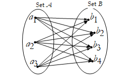
Figure 2.3. The Cartesian Product of two sets.
The arrows show how we combine the elements in pairs. The Cartesian product for these sets is then,
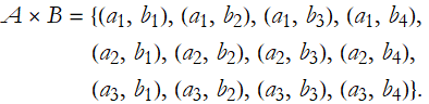
(2.15)
Journeyman Exercise 2-2: Invent two sets with two or three elements each and write out the Cartesian product of the two.
Journeyman Exercise 2-3: Can we have a Cartesian product of three or more sets? Interpret what that Cartesian product would tell us.
We can formally state that a relation is a subset of the Cartesian product of the sets,
![]()
(2.16)
The thing to realize, as we have seen for the set combinations given above, is that R is replaced by some symbol. For example, we can use the equal sign as a relation, we write a = b, this is called the Identity Relation. We can see that an Identity Relation limits the elements of the Cartesian product that conform to the relation, thus it is a subset of that Cartesian product.
In a relation R⊆A×B the set A is called the domain of the relation and B is called the range of the relation. If A=B, then we say that R is a relation on A.
Getting back to the identity relation, we can write this more formally
![]()
(2.17)
Apprentice Exercise 2-8: Translate (2.17) into its English equivalent.
Let’s say that we take three elements of a set A: a, b, and c. Let’s also say that we have some generic relation on A, called R. If for every a∈A, such that we can write a R a, then we say that R is a reflexive relation.
If a relation is not reflexive, it is said to be irreflexive.
![]()
(2.18)
where we can use the symbol ¬ to represent not, then we rewrite this,
![]()
(2.19)
Apprentice Exercise 2-9: Translate (2.19) into its English equivalent.
If for every a∈A and for every b∈A where we write a R b implies b R a, then we say that the relation is symmetric. Note that this gives us the first mathematical expression for symmetry. Here we see that the relation remains the same no matter which order we place the symbols being related,
![]()
(2.20)
Apprentice Exercise 2-10: Translate (2.20) into its English equivalent.
If for every a∈A and for every b∈A and for every c∈A, if we write a R b and b R c implies a R c, then we say that the relation is transitive.
![]()
(2.21)
Apprentice Exercise 2-11: Translate (2.21) into its English equivalent.
Any relation that is reflexive, symmetric, and transitive is called an equivalence relation.
Journeyman Problem 2-4: Prove that = is an equivalence relation.
In this way we can state that a function is a relation. Given that a∈A and b∈B, then the function f where b=f(a) implies that f:A→B. Here the set B is called the codomain of the function. If f:A→A, the domain and the codomain are the same set, then we can call f an operator. The subset of the codomain that form the specific values of the function is called the range of the function.
If you have a function with two independent variables, a and b, where a≠b implies that f(a)≠f(b) tells us that the function is classified as injective (also called one-to-one).
If you have a function where every element of the codomain has a corresponding unique element in the domain then we classify the function as a surjection (also called an onto function).
If a function is classified as being both injective (one-to-one) and surjective (onto) then it is said to be a bijection (also called a one-to-one correspondence).
Functions and Cartesian Plots
Now we know what a function is, what do we do with one? It turns out that in order to use a function we need a way to represent the values of the independent and dependent variables. There are three ways to do this. The first way is to establish a table where we put the independent variable values in one column and then list the correlated dependent variable values in another. A second method is to produce a formula that represents the rule of the function, as we have done in Apprentice Exercise 2-1 above. A third method is to produce a graph, or plot, of the function.
You may recall from high school mathematics that we can correlate a line with numbers, thus representing numbers as positions along a line, (see Fig. 2.4).
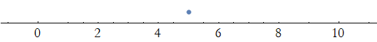
Figure 2.4. The number 5 represented on a number line..
We can have two number lines. One representing the independent variable is called the abscissa. Most often this is placed so that the line is horizontal. Another representing the dependent variable is called the ordinate, and is placed vertically and perpendicular to the abscissa (see Fig. 2.5).
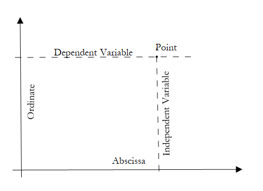
Figure 2.5. The coordinate system forming a plane.
Such an arrangement is called a Cartesian Plot, or, since it is two-dimensional, the Cartesian plane. You find the independent variable along the abscissa, then you find the dependent variable value along the ordinate. You place your point at the intersection.
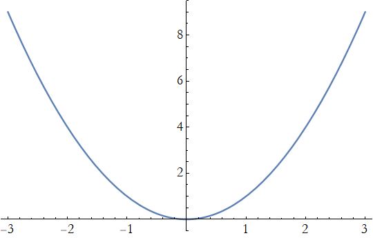
If there is a table of function values you can plot each point. Here is an example of a table of points for the function ![]() .
.
| x | y | |
| -3. | 9. | |
| -2.75 | 7.5625 | |
| -2.5 | 6.25 | |
| -2.25 | 5.0625 | |
| -2. | 4. | |
| -1.75 | 3.0625 | |
| -1.5 | 2.25 | |
| -1.25 | 1.5625 | |
| -1. | 1. | |
| -0.75 | 0.5625 | |
| -0.5 | 0.25 | |
| -0.25 | 0.0625 | |
| 0. | 0. | |
| 0.25 | 0.0625 | |
| 0.5 | 0.25 | |
| 0.75 | 0.5625 | |
| 1. | 1. | |
| 1.25 | 1.5625 | |
| 1.5 | 2.25 | |
| 1.75 | 3.0625 | |
| 2. | 4. | |
| 2.25 | 5.0625 | |
| 2.5 | 6.25 | |
| 2.75 | 7.5625 | |
| 3. | 9. |
Assuming that the values of one column, in our example x, correspond to points on the abscissa and values from another column, in our example y, correspond to points along the ordinate. Here is an example of such a plot of points for our example.
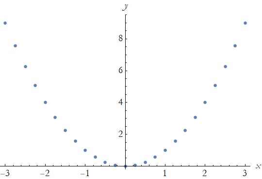
Figure 2.4 A plot of values from a table.
If you have enough points you can connect them by smooth curves and produce a plot of the curve of the function. Here is an example of such, based on the previous example.
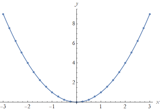
Figure 2.5 A plot connecting the points of the previous plot by a smooth curve..
So we have identified two methods of describing functions; making a table of their values, and making a plot. Such descriptions are called representations. As it happens we can also represent functions using equations. For example, we used ![]() as the equation representing the function.
as the equation representing the function.
Models—Equations Representing Functions
There is a school of thought that physics requires that you set up, study the behavior of, and solve equations. When you search through a set of data you might note the existence of a pattern. This pattern might suggest an equation. This sensed equation is a representation of a possible function relating the data. By understanding the behavior of this function, we might learn to understand the behavior of the data and the underlying processes that generated the data. If we make the assumption that the equation we perceived in the data is true, we can try to solve that equation for different situations of the independent variable. This solution is a prediction of the outcome of an experiment where the specific independent variable is adopted in a laboratory. Such a prediction is called a model. Many theoretical physicists spend their entire careers making models to try to understand specific physical phenomena.
How do we construct a mathematical model of a physical phenomenon?
Find or construct a mathematical representation suitable for your subject.
Modify this representation to suit the phenomenon you are studying.
Decide on a representation style you want for your prediction.
Vary the independent variable(s) as seems reasonable for what you want to model.
To do all of these things you will need a lot of experience. That is why doing problems is important. You will need to increase your mathematical skills and your physical intuition. Remember that there is no way to prove that a model is physically viable. You can show that a model is not viable. The best you can ever say about a model is that it is consistent with the data.
How do you get experience in making models? There are two pathways that we will pursue at the same time. The first is to develop mathematical language and techniques to shape our models into such language. The second way is to develop mathematical representations of the subjects of physics that can be adapted using mathematical techniques and physical intuition and argument to specific problems. The rest of this chapter will consist of examining different functions and the capabilities that they give us.
The first kind of function we will examine is one whose plot results in a straight line. Wait, what is a straight line? There are two properties that we can check to make sure something is straight. If we draw a line, like this,
![]()
Figure 2.6 A line segment.
the first test would be to flip the top and bottom and make sure it still looks the same.
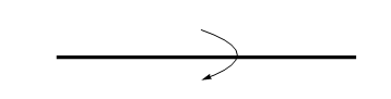
Figure 2.7 The mirror symmetry of a line segment.
Any time that we can do something to an object and it looks the same after we did it, we call that a symmetry. Symmetries are very important to physics, it turns out that all of the conservation laws of physics are the result of symmetries. The symmetry we have just seen would result if we took a mirror and placed it along the line. Thus we can call this a mirror symmetry. The second test of straightness occurs if we can find a symmetry after rotating the line 180° about an imaginary line extending toward you from the center of the segment.
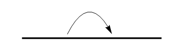
Figure 2.8 The symmetry of a line segment after a 180° rotation.
Any segment that meets these two symmetries is called straight.
What sort of function results in a plot of a straight segment? If we examine the segment of the three diagrams above we can conclude that the equation will just be
![]()
If the segment is not located on the x-axis, but is some height above the axis, represented by b, then we can change the equation to
![]()
If the line as at some angle, in other words it is no longer parallel to the x-axis, then we need to figure out how to write that.
Figure 2.9 A line segment at an angle from the horizontal.
We can establish two points along the segment, ![]() and
and ![]() .
.
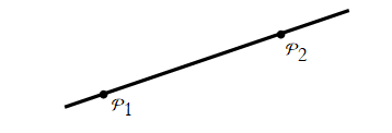
Figure 2.10 Two points on a line segment at an angle from the horizontal.
We can establish the distance between the x-values of the two points,
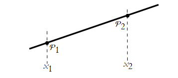
Figure 2.11 The distance between two points on a line segment in the x-direction.
where we can calculate the distance in x and call it the interval of x, denoted Δ x. Note that this is not Δ times x. For formula we use is,
![]()
(2.22)
We can do the same thing for the y direction.
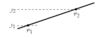
Figure 2.12 The distance between two points on a line segment in the y-direction.
Where the y-interval is then given by
![]()
(2.23)
The ratio of the intervals gives us the angle and it is called the slope of the line, or the gradient of the line. We can denote this as m, and write
(2.24)
Our equation is then almost complete, except that b takes on a new value. It is now the the value of y when x is equal to 0, and is often called the y-intercept. We can then write the generic equation of the line
![]()
(2.25)
Such equations are called linear equations, or equations of the first-degree. The degree here represents the highest power of the independent variable. A function represented by such an equation is called a linear function.
Apprentice Exercise 2-12: Make up the slope and y-intercept from (2.25) and make a table of values of y given x. Plot this curve. How many times does the curve cross the x-axis (this is where y=0)? Such an x-intercept point is called a zero of the equation. A zero is sometimes called a solution or root of an equation.
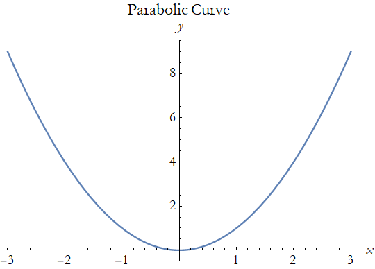
So, what is a second-degree equation? By the definition of degree that we have covered it is an equation involving a factor of the square of the independent variable. This is often called a quadratic equation and it has a general form involving a generic coefficient a and some constant added in, b, this constant will determine how far above the lowest point of the curve is above the x-axis,
![]()
(2.26)
Any function represented by this equation is called quadratic function.
Apprentice Exercise 2-13: Make up the coefficient and constant from (2.26) and make a table of values of y given x. Plot this curve. Identify the curve. Is there a zero to your equation? What do you think is the maximum number of zeros of a quadratic equation?
All equations involving positive integer powers of the independent variable are called polynomial equations. If the highest power of the independent variable is n then the corresponding equation is called an nth-degree equation. Such an equation has a collection of n coefficients ![]() and the equation has the form
and the equation has the form
![]()
(2.27)
Apprentice Exercise 2-14: Choose a degree for your equation. Make up the list of coefficients from (2.27) and make a table of values of y given x. Plot this curve. What do you think is the maximum number of zeros?
Journeyman Problem 2-5: In general for an nth-degree equation, how many zeroes are there?
When we take the square of a number, the answer is always positive. It matters not that the base is negative. Thus, when we take the root of a positive number, the answer must almost always be in the form of a pair, a positive number and a negative number.
What happens if the square is a negative, number? We cleverly choose the symbol i to represent this case,
![]()
(2.28)
or
![]()
(2.29)
The symbol i is what we call the imaginary unit and any product of a real number with the imaginary unit is called an imaginary number. In engineering, the imaginary unit is often given the symbol j.
Apprentice Exercise 2-15: Evaluate ![]() .
.
Apprentice Exercise 2-16: What are the first four powers of i?
One way of defining a complex number, z, is to say it is the sum of a real number, say x, and an imaginary number, say i y,
![]()
(2.30)
This is called the Cartesian form.
When we replace i by -i, we have the complex conjugate of z, and we write this ![]() .
.
![]()
(2.31)
Journeyman Problem 2-6: When is a complex number equal to its complex conjugate?
We can think of x as being the real part of the complex number, z, denoted Re(z). Then y would be the imaginary part, denoted Im(z). In this way we can also think of a complex number as an ordered pair of real numbers, z=(x,y).
What operations can we perform with complex numbers? Let’s say we have two complex numbers,
(2.32)
then their sum is
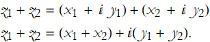
(2.33)
Apprentice Exercise 2-17: How do you subtract complex numbers?
The product of two complex numbers is similar to how we multiply two polynomials,
![]()
![]()
![]()
![]()
(2.34)
Apprentice Exercise 2-18: Evaluate ![]() .
.
The quotient of two complex numbers is,
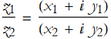
(2.35)
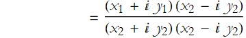
We can represent complex numbers graphically. The process for this is identical to the way we represent points on the Cartesian plane. The real part is located on the horizontal axis, and the imaginary the vertical. Thus a point defined by z=x + i y and its complex conjugate are represented in Figure 2.12.
Figure 2.12 The Argand Diagram for a complex number and its conjugate.
This representation is called an Argand Diagram, named for Jean-Robert Argand (1768-1822), but is really due to Caspar Wessel (1745-1818).
Complex numbers add and subtract just as if they were arrows, the prototype of vectors. You place the tip of one vector on the tail of the other.
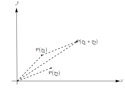
Figure 2.13: The Argand Diagram for the sum of two complex numbers.
It is important to realize that the coefficients in (2.27) may be complex. With that in mind, and with the results from Journeyman Problem 2-5, we can state the following theorem:
Theorem 2-1: A polynomial of the nth degree having complex coefficients will have n complex roots.
This leads us to the Fundamental Theorem of Algebra:
Theorem 2-2 (Fundamental Theorem of Algebra): Every polynomial of positive degree having complex coefficients has at least one complex root.
Journeyman Problem 2-7: How do we reconcile Theorems 2-1 and 2-2?
We can write two polynomials along the lines of (2.27),
![]()
(2.36)
and
![]()
(2.37)
so we can define a new type of function,

(2.38)
this type of function is called a rational function.
Apprentice Exercise 2-19: The simplest rational function is represented by the equation  . Make a table of values for this equation and plot it. Speculate on what happens when x=0.
Trigonometry
We have all seen right triangles in high school math. Figure 2.14 is a prototypical right triangle with the altitude marked as a, the base marked as b, the hypotenuse marked as c, and the angles marked as theta θ and phi φ.
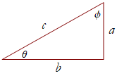
Figure 2.14: A right triangle with segments and angles indicated.
We can define the functions sine (sin), cosine (cos), and tangent (tan), as ratios of the various sides according to the following relationships:
![]()
(2.39)

(2.40)
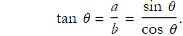
(2.41)
There are a couple of useful things to know about the trigonometric functions. The first is that we can draw a triangle within a circle, with the center of the circle located at the origin of a Cartesian coordinate system, as in Figure 2.15
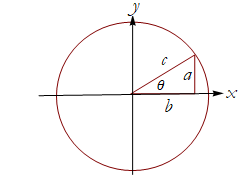
Figure 2.15: A right triangle drawn in a circle.
If this circle has a radius of 1 unit of length, then we call it the unit circle.
In physics we do not generally use the degree as a measure of angle. Instead we use the radian; we say that there are 2 π radians in 360°, or 1radian=π/180°, thus 90°=π/2 radians, and 30°=π/6 radians. Thus a radian is about 57° (see Figure 2.16).
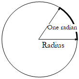
Figure 2.16: The radian as the angle subtended by an arc equal to the radius of the circle.
So a trigonometric function on the unit circle is sometimes called a circular function. This is one reason why trigonometric, or circular, functions always seem to have values from 0 to 1. Here the line connecting the center of the circle to any point along its circumference forms the hypotenuse of a right triangle, and the horizontal and vertical components of the point are the base and altitude of that triangle. The position of a point can be specified by two coordinates, x and y, where
![]()
(2.42)
and
![]()
(2.43)
This is a very useful relationship between right triangles and circles.
Now, suppose that a certain angle θ is the sum or difference of two other angles using the Greek letters alpha, α, and beta, β, we can write this angle, θ, as α±β. The trigonometric functions of α±β can be expressed in terms of the trigonometric functions of α and β.
![]()
![]()
![]()
![]()
(2.44)
There are many other such useful relationships. We will examine one more here,
![]()
(2.45)
Notice the notation used here: ![]() . This equation is the Pythagorean theorem in disguise. If we choose the radius of the circle in Figure 2.15 to be 1, then the sides a and b are the sine and cosine of θ, and the hypotenuse is 1. Equation (2.45) is the familiar relation among the three sides of a right triangle:
. This equation is the Pythagorean theorem in disguise. If we choose the radius of the circle in Figure 2.15 to be 1, then the sides a and b are the sine and cosine of θ, and the hypotenuse is 1. Equation (2.45) is the familiar relation among the three sides of a right triangle: ![]() .
.
Solving Equations
I assume that you know how to solve equations from high school math or your own independent study. For completeness, and because it is very important to physics, I will go over the basic ideas.
Given an equation, say (2.25)
![]()
the goal is the find an expression for x in terms of y. To do this we use progressive inverse methods to isolate x. We begin with subtraction. When we perform one operation on an equation it must be applied to both sides. We subtract by b,
![]()
![]()
The we divide by m,
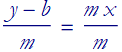
![]()
so we have solved the generic linear equation for x,  .
.
Algebraic Manipulations and Functions in Mathematica
Everything in Mathematica is treated as an expression. It is a good idea to label every expression so you can refer to it later. I use exp1, exp2, and so on.
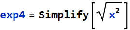
There are two powerful commands for simplifying expressions. The act of simplification is a set of transformations that result in the simplest for of the expression. The first is Simplify[expression]. Here we have a simplification of a polynomial.
![]()
![]()
Note that the order is reversed from the way most of us would write it. We can use the // to put a command at the end of the instruction. We can use the instruction TraditionalForm to write the answer in a nice font and in a way that matches how we might write on a note pad.
![]()
![]()
Here we have a rational expression.


Sometimes we will need to make assumptions clear before getting the answer we want. Here is an example.
![]()
While this is true, it is not very useful. We note our assumption that x∈R,
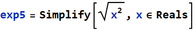
![]()
That’s better.
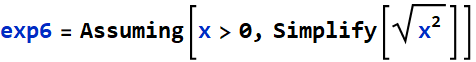
We can also use the Assuming command first,
![]()
FullSimplify an be used if Simplify is not effective. Warning FullSimplify takes more time.
![]()
![]()
Expand allows you to expand products and integer powers. For example.
![]()
![]()
![]()
![]()
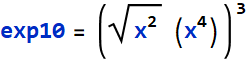
PowerExpand allows you to expand all products of powers and powers.
![]()
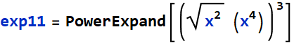
![]()
We can use ExpandAll when we have a combination of sums and powers.
![]()
![]()
ComplexExpand allows us to expand complex expressions. Here we see the results for a complex polynomial.
![]()
![]()
![]()
![]()
Factor allows us to factor a polynomial.
![]()
![]()
Collect[expression,form] collects terms of powers that match the form specified.
![]()
![]()
We can simplify this,
![]()
![]()
Together places the terms into a sum over a common denominator


Refine allows us to convert a symbolic expression to one where a numerical factor would be included, returning to an example from above we see
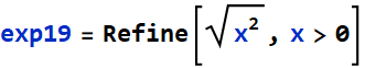
![]()
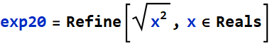
![]()
Distribute allows us to apply the distributive law over an operator, in this case multiplication,
![]()
![]()
Distribute does not perform the addition in the correct order, so the product disappears.
![]()
![]()
To do it correctly we can use the command Unevaluated around the product, this allows the product to be done in the correct order.
![]()
![]()
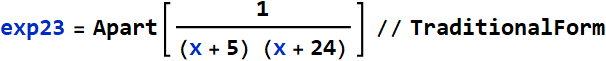
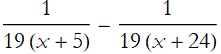
Apart makes a rational expression into a sum of minimal denominators,
Trigonometry and Equations in Mathematica
The plot command plots an expression for an independent variable over a specified range of values.
![]()
We can easily make this plot useful to all viewers by labeling the axes with nicely formatted labels, and providing a label for the plot itself. Show allows us to combine many graphics command into a single unit. GrayLevel->0 is the value for black.

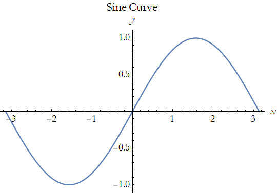
Here we show how Mathematica handles a trigonometric function.
![]()
Here are some examples of trigonometric expressions, these apply relevant trigonometric identities.
![]()
![]()
Simplify does this automatically.
![]()
![]()
PowerExpand does not,
![]()
![]()
instead we use TrigExpand
![]()

TrigReduce should reverse the expansion.
![]()

Why did it fail? TraddiationalForm is the problem. How do we get expressions to work correctly and display the way we want them to? Wrap the TraditionalForm around the expression instead of applying it at the end.
![]()

this does not change the expression,
![]()

![]()
Mathematica can symbolically solve equations, note that the result is in the form of a transformation.
![]()
![]()
We can remove a level of brackets by specifying the first solution.
![]()
![]()
Or we can tell Mathematica to display the solution and transform the symbol for x according to the solved equation.
![]()
![]()
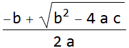
We can reproduce the quadratic formulas.
![]()
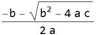
![]()
Mathematica can solve systems of equations, too.
![]()
![]()
![]()
![]()
![]()
![]()
Or we can perform a real approximation of these exact results,
![]()
![]()
![]()
![]()
Reading List
1. Bruce Meserve, (1953), Fundamental Concepts of Algebra, Addison-Wesley Publishing Company, reprinted in 1982 by Dover Publications. This is probably my favorite book on elementary algebra. I also like its companion volume by the same author Fundamental Concepts of Geometry.