Chapter 1: Physics

George E. Hrabovsky

Theoretical Physics in Brief

I will begin by assuming that you have had some high school science and mathematics. I am not going to assume that you have mastered all of it, just that you will be able to follow me when I ask you to recall some basic points of algebra or geometry. As you proceed through this book I suggest you try every problem. Those identified as Apprentice level will have detailed instructions to guide you. Those listed as Journeyman will have few instructions, since it is assumed that you have all of the necessary background to perform it, or that you will wait to work on it until you do. Master level problems will have no instructions and may be research level problems that may not even have a known answer.

To start talking about theoretical physics we must begin by talking about science. We understand science to be very powerful and most people are highly respectful of it. What makes our respect for it so high? Why do some people distrust it?

In one sense science is a process. It describes the actions of the scientist. How observations lead to the perception of patterns. Adopting such patterns as reality leads to predictions. How predictions are tested against experiments in the laboratory, or chance observations in nature. In this way science is an activity.

The facts that are the product of the activity of science is what we call the body of science. Here is something to remember though: We might slice up the body of science into physics, chemistry, enzymology, and so on, nature does not know anything about such divisions. There are many examples of synergy between previously disconnected areas of science (for example the recent ideas that information might be fundamental to physics).

Apprentice Exercise 1-1: A laboratory experiment, in principle, allows us to recreate nature where we are in control of the environment and all aspects of the lab that are relevant. If we assume that experiments can be conducted carefully, so that principles tested against such experiments can be trusted, what confidence in the validity of the principles should we give? Under what circumstances should we withhold our trust in such a situation? Can this situation ever be achieved in reality?

Apprentice Exercise 1-2: If an experimental result indicates that a long-held scientific principle is wrong, what should we do? What does this imply abut the nature of scientific principles?

Apprentice Exercise 1-3: Observing nature, especially at a distance, is less trust-worthy than a careful experiment. Why is this? What can we do to make such observations more reliable?  Can they ever be as reliable as an experiment? Since sciences such as ecology, meteorology, astronomy, and the like are mostly based on observations, what does this imply regarding their results? Does this ever mean that we can just ignore their results?

Apprentice Exercise 1-4: Can science be applied to every field of study? Can you think of a situation where even observations cannot be performed to verify results?

So, what is physics? Like science in general, physics can be thought of as a process. We find the use of high precision instruments allow us to make detailed observations. Advanced data analysis methods allow us to identify patterns. Advanced mathematical and computational methods allow us to make detailed predictions. And high technology laboratories allow us to test these predictions. In short the methods of physics are the best examples of the process of science.

The noun of physics is vast. There are hundreds of web sites, thousands of books and hundreds of thousands of research papers containing the lore of physics.

This book will not discuss in any but a cursory fashion the ideas of observational or experimental physics. We will show some methods of data analysis as we need them. This book will explore in detail the mathematical and computational methods applied to develop theoretical physics, but only as we need them.

So, what is theoretical physics? At first glance, and we will spend a lot of time taking such glances, theoretical physics serves to make predictions of the basic principles that can be tested. Such a prediction is called a model and it can be mathematical or computational. A mathematical model requires a mathematical formulation of a physical principle to make the prediction. A computational model requires a computer-based formulation of the physical principle to make the prediction.

So the choice of mathematical/computational formulation is important. So, the second glance at the nature of theoretical physics is the development of such formulations. We need to be able to use the methods of mathematics to prove that our formulations are internally self-consistent. This leads to a third glance, redefining the noun of physics in terms of any new formulation you develop.

Once you have a formulation, the fourth glance is the ability to apply it to the physical situation you are trying to predict. Most often you choose to view one aspect of the situation as depending on another aspect (say the location of an object might depend on the passage of time). How is the first aspect dependent on the second? Another way to ask it is, “How does the first aspect change with respect to the second aspect?” In the example we invented, this might be restated, “How is the location of an object changed by the passage of time?”

It turns out that there is an entire field of mathematics that allows us to study such changes and their ramifications. It is called calculus and we will spend a lot of time on it. We will develop calculus ideas and methods as we need them. A systematic approach to this field is far beyond the scope of this book.

The result of applying calculus to make a prediction is most often a special kind of equation that described the physical situation. There are many methods for writing and solving such equations, and we will spend some time on both, though it is not possible to develop a systematic presentation of such methods in this book. We will develop any methods we need as we go.

For simple situations we can derive the equations of physics using the principles of calculus. As we incorporate complexities into our models we will reach a view when aspects of the system cannot be represented by simple numbers. Instead they take on the character of arrows. Such a representation eventually leads us to the ideas and methods of vector analysis. Again we will use these ideas as we need them, but we will not develop them in any systematic way. The application of vector analysis, for a time, allows us to simplify our results.

At some point the vector formulation begins to make things more complicated again. While understanding how we use vector analysis is easy, actually using it can become nightmarishly difficult.

It turns out that we can construct a new aspect of the situation that was previously hidden that we call the action of the situation. We can use a new mathematical field called the calculus of variations to impose a condition that the action will not change. To do this we reformulate the situation so that all we need to know are where it is located at the beginning and at the end. This is called the variational formulation, and we can rewrite all of physics using it. Deriving this formulation can be difficult to understand, but using it is very easy. Thus we have a method to get the necessary equations for even vastly complicated situations in a very straightforward way. We will develop and use variational methods as we proceed, but it is beyond the scope of this book to present a systematic treatment of it.

It All Starts with Measurement

Let’s say you want to study the motion of a car. There are the components of the engine moving and exchanging fluids, the wheels rotating and bending, people inside the car moving and breathing, the car itself moving on the road and creating turbulence in the air as it passes. This is a very complicated situation, despite our familiarity with it.

Imagine that you can zoom out so that you can avoid most of this complexity. You no longer see the internal workings of the car. You have the same situation, but it's a simpler picture. We have abstracted away a lot of complications.

Imagine that you zoom out till all you see is a speck in the distance. This speck still has all of the properties of the car that we started with. All of the internal systems are still there. We just don't need to worry about them.

Now we have to make a leap of faith. We have to believe that we can treat an object as if we were a zoomed out speck. Think about what we are losing by treating the object as a speck. The first thing we lose is all of the internal complexities of the object. We also lose the size and shape of the object. Whenever we have an object where we do not need to worry about its size, shape, or its internal workings we can look at it as if it were a speck. Such a simplified object is called a particle. The highest level of abstraction for an object of any kind is to treat it as if it were a single particle, even though we know that no object is really a particle.

The drawback is that by removing the complexities you also remove levels of reality. So what is the point of the abstraction? It makes the problem simple enough to start developing a mathematical or computational formulation of it. Once you understand the simplified formulation, you can begin to put the complexity back to make it more realistic. This process of abstraction is the heart of theoretical physics.

For our purposes a system has one or more particles along with one or more rules that determine how the system changes. Of course, the simplest possible system is a single particle whose rule is that it never changes. This is both simple and it is also incredibly boring. The list of properties that uniquely determines everything we need to know about a system is called its state. Another word for the state of a system is its configuration.

Most often we attempt to represent the state of a system as a set of numbers. These numbers represent the relevant physical properties of the system. If these properties are subject to change, we can call them state variables. If the properties are not subject to change they are called physical constants. If the properties are fixed for a given situation, but may change from one situation to another, we will call them physical parameters.

A physical quantity that does not change with a corresponding change in size is called an intensive quantity. On the other hand, a quantity that is additive among all of the subsystems of a larger system (thus the quantity of the larger system is the sum of the quantities of the smaller subsystems) is called an extensive quantity.

Journeyman Problem 1-1: We have briefly discussed systems of particles. Are there other kinds of systems that might not involve particles? If so, can you explain what you are thinking about with regard to such systems?

Broadly, there are two types of systems. A system that does not allow new components to come in or existing components to leave is called a closed system. A system that allows components to come and go is called an open system.

The simplest state variable is the location of a single particle. We must be able to locate a particle. To that end we state these facts:

We will understand that everything we are interested in is happening in a place. We will call this place a space. An example of space is physical reality. Another example is a list of all possible states a system can be in, this is a state space.

Our space can have regions within it that we will call subspaces. Each such subspace can be thought of as a state.

One class of such subspaces has no size or shape, this is called by the term point.

Given the fact that the point has no size or shape, and a particle is considered without regard to size or shape, we can say that a point is a mathematical representation for the location of a particle.

This reduces our problem to finding a point representing the location of a particle within a space. The first thing to realize is that we cannot find the position of anything without knowing what that position is relative to. In other words, we have to identify some arbitrary reference point. We will call this reference point O. This is the classical notation for the origin. You can think of the origin as a place to start. We can also set a point representing the location of the particle, called P (see Figure 1.1).

Figure 1.1: The origin and the location of a particle.

We now recall from basic geometry Euclid's First Postulate: For every point O and every point P not equal to O there exists a unique line that passes through O and P. This line is denoted .

Any two points, O and P, and the collection of all points between them, that lie on the line combine to form a line segment. Our segment is denoted (Figure 1.2).

Figure 1.2: The line segment .

The segment   is called the distance between O and P. We can measure this distance, denoted D(OP).

Recall from basic algebra that, given a number x the absolute value of x is x itself so long as x is greater than or equal to 0; if x is less than 0 then its absolute value is -x. Symbolically we write it this way:    

(1.1)

The Ruler Axiom of geometry states: Given a line  , there exists a one-to-one correspondence between the points lying on the line and the set of real numbers such that the distance between any two points on is the absolute value of the difference between the numbers corresponding to the two end points. From this we can construct another expression for distance by applying the definition of the absolute value to the Ruler Axiom and then to the definition of distance we get,

(1.2)

To measure this we have to establish a unit of length. Let us say that this is a segment bounded by the points and (see Figure 1.3).

Figure 1.3: Applying a unit length segment.

We next have to find a point on such that (see Figure 1.4),

Figure 1.4: Finding the point .

If we repeatedly apply something, we call it an iteration. We apply the unit length iteratively until we have n equal segments (see Figure 1.5).

Figure 1.5: Finding the successive points.

And thus the distance for the segment is then,

(1.3)

Thus, measuring distance is the iterative application of a unit of length n times and then adding any fractional remainders.

We can't discuss a practical measurement without including the unit of measurement we are using. In this way the length of the segment becomes an algebraic quantity with the number of units being the coefficient of the symbol for the unit. We might say four feet, or ten point three six meters, or six and a half light years, etc.

In the abstract we can assume that we are talking about arbitrary units, and so will implicitly understand that units are being considered without stating it.

Apprentice Exercise 1-5: If we were to consider the time measured on a clock to be a real number, construct a line segment that represents the duration of an experiment. Subdivide this line segment by applying a unit of time in the same way as we did for distance. Derive a formula similar to Equation (1.3) for the total duration of the experiment.

Apprentice Exercise 1-6: We understand weight to be the influence of gravity acting on the mass of an object. We understand mass to be a measure of the quantity of substance an object has. This is necessarily a naive and imprecise way to think about mass, but it is the best we can do for now. Derive a formula similar to Equation (1.3) for the mass of a particle.

Apprentice Exercise 1-7: We understand temperature to be a measure of the collective motions of the atoms within an object. Derive a formula similar to Equation (1.3) for the temperature of an object.

If we have a large distance, like 10,000,000,000 miles, is there an easy way of writing and calculating with it? Yes there is. We accept the left-most place value as the leading digit and write that down as if it were the one’s place value, then we write any necessary value as a decimal fraction. Then we multiply by the necessary powers of ten to get to that decimal value. For example, we would have 1 as our leading digit, there are no decimal fractions, and we have ten powers of ten. So we would write it as miles. If instead we had 12,517,000,000 miles, we would write it miles. If we keep in mind the rules regarding exponents this makes such calculations fairly easy. This is called scientific notation.

Short distances are handled the same way, except we use negative powers of ten. So, the distance of 0.00000000000001 meters becomes meters.

So what are the standard units for the physical quantities we have introduced so far? There are several systems of units to choose from. There is the English system, ironically no one in the world other than the US uses this system. There is the SI, or metric, system (SI stands for System International). There is the Gaussian (it is pronounced gows-eean and is also called the cgs system).

Perhaps the most natural thing to measure is the distance between two points. In the English system length is presented in a bizarre system that those of us in the United States find natural. The starting level is the inch (abbreviated in), we also have the foot (abbreviated ft), the yard (abbreviated yd), the mile (abbreviated mi), and the  nautical mile (abbreviated nm). The SI system uses the meter (abbreviated m). The Gaussian system uses the centimeter (abbreviated cm).

The units of time are seconds (abbreviated sec), minutes (abbreviated min), hours (abbreviated hr), and years (abbreviated yr) all of which are in the English system. The unit of length in the SI system is the second. The unit of time in the Gaussian system is also the second.

The unit of mass is either the pound (abbreviated lb) or the slug (abbreviated sl) in the English system. The unit of mass in the SI system is the kilogram (abbreviated kg). The unit of mass in the Gaussian system is the gram (abbreviated gm).

The units of temperature are degrees Fahrenheit (abbreviated °F) in the English system. The unit of temperature in the SI system is either degrees Celsius (abbreviated °C) or Kelvin (abbreviated K). The unit of temperature in the Gaussian system is either the degree Celsius or the Kelvin.

Position is represented by a real number, and we write it x∈R. The problem is that almost all real numbers can only be written as decimal approximations. Thus there is some uncertainty as to exactly where a particle is located. We also gain some error in the measurement process itself, we almost never have a perfect fraction of a unit when we measure something. We can only approximate such a position. This is what we call measurement error.

This uncertainty in measurement will grow with repeated measurement. This is called the propagation of error.

Journeyman Problem 1-2: Speculate on the effect of the propagation of error with successive time measurements.

As long as you have the same kind of quantity you can convert one unit into another. Inches can become feet, feet can become meters, and so on. This is called unit conversion.

Apprentice Exercise 1-8: Make a table of unit conversions between inches, feet, yards, miles, meters, and centimeters. Make a table of unit conversions between seconds, minutes, hours, and years. Make a table of unit conversions between pounds, slugs, kilograms, and grams. Make a table of unit conversions for degrees Fahrenheit, degrees Celsius, and Kelvin. Now make up a distance, a time, a mass, and a temperature and determine their respective values in each unit.

Rules of Algebra

This section is not so much a review of algebra, I assume that you have studied algebra elsewhere. I simply thought it would be useful to list the most important and useful tricks used in manipulating algebraic expressions. I may comment on a rule, but I will likely just write a rule down along with its name.

Commutative property of addition

(1.4)

Commutative property of multiplication

(1.5)

Associative property of addition

(1.6)

Associative property of multiplication

(1.7)

Additive inverse

(1.8)

The additive identity is 0

(1.9)

You can always add any expression whose value is zero to any expression when it is in the form of (1.8). Say you have and you want , if you add x-x it gets you closer to what you want .

Left-distribution

(1.10)

Right-distribution

(1.11)

The reciprocal of a non-zero real number

(1.12)

Multiplying a rational expression

(1.13)

The multiplicative identity is 1

(1.14)

You can always multiply any term by any expression that equals 1. You can always multiply any term by an expression similar to (1.10) in the form (1.11). Let’s say you have an expression y/x and you want , then you multiply by x/x to get and that gets you closer to what you want.

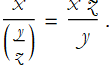
Dividing a rational expression

(1.15)

Dividing by a rational expression

(1.16)

Dividing a rational expression by a rational expression

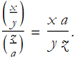
(1.17)

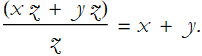
Adding or subtracting rational expressions

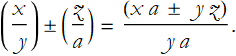
(1.18)

Expanding a rational expression

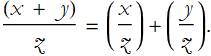
(1.19)

Cancelling a rational expression

(1.20)

The exponential identity

(1.21)

Multiplying exponents of the same base

(1.22)

Dividing exponents of the same base

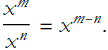
(1.23)

Raising a power by an exponent

(1.24)

Expanding a product raised by an exponent

(1.25)

Expanding a rational expression raised by an exponent

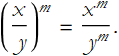
(1.26)

The reciprocal power

(1.27)

A rational expression raised to a reciprocal power

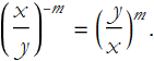
(1.28)

The power equivalent of a radical

(1.29)

Magic I: Estimating Physical Quantities

So you are beginning a study and find that you need the value of some physical quantity. You look it up and can’t find that value. What do you do? You can’t simply give up. The answer is that you make a guess of the value you are looking for. If you are careful we no longer call it a guess, we call it an estimate.

John Archibald Wheeler (1911-2008) was one of the most influential theoretical physicists of the twentieth century. In his book with Edwin Taylor, Spacetime Physics he gives a lot of good advice to students just beginning to study relativity. I will now introduce the notation for references that we will use in this book. When you see the symbol [1], it means reference number 1 for the current chapter, and [1-1] is reference 1 from chapter one. The book by Taylor and Wheeler is [1]. It is a wonderful book introducing relativity. There is one part that is particularly useful to our work. Here we begin a discussion of it.

“Wheeler’s First Moral Principle: Never make a calculation until you know the answer.” This seems kind of silly. Is it a mere aphorism? The condition for knowing the answer can be somewhat relaxed to mean until you have an good idea of what the answer will look like. “Make an estimate before every calculation,” makes this explanation clear. “Try a simple physical argument before every derivation,” a physical argument is one that calls upon knowledge and/or intuition of the physical situation, possibly based on experience of calculations and study.

So this is great! All you have to do is make an estimate, right? So how do you make an estimate? What, exactly, is an estimate? It turns out that an estimate is a guess or rough approximation of a calculation. This does not mean that it is not done carefully. Unless you are dealing with a problem that is trivially easy, you will probably apply one or more of several methods.

Make an initial guess, this can lead you to a more precise strategy.

If you know them, or can quickly look them up, apply common values of physical quantities.

Look at your initial guess and decide if it is close.

Break a complicated problem into pieces that you can attack on their own. This is called the method of divide and conquer.

Do the easy parts first.

Look up facts related to your problem to make the estimate.

If you need to know some fact that you don’t know, assume the nature of the fact and use that assumption.

If there is a complicating factor (this is just some factor that complicates things), remove that factor in the first estimate and see if the result gives you a clue as to how to deal with it.

Invent notation for complicating factors and see if that symbol gets removed along the way.

Apply the idea of proportionality. If it doesn’t seem to apply, then drop it at first. You can always come back to it later.

Change the scale of the system and try to figure out how the quantities of interest change with such scale changes. If a quantity does not change with such a change of scale it is called an intensive quantity.

Try to use intensive quantities when applying a scaling argument, that way you have fewer things to change.

See what happens when you choose extreme cases (0 or ∞) as values for a significant quantity. Be sure to use the solution you get to check the validity of the application of the extreme case.

Use more than one method and see if you get the same answer.

Apprentice Exercise 1-9: Estimate the thickness of a sheet of paper. You can begin by determining the thickness of a certain number of sheets of paper. Then you can divide that by the number of sheets.

Journeyman Problem 1-3: Estimate the number of hairs on the average head.

Magic II Dimensional Analysis

Not all units of measurement are direct. Some are composed of several other units combined in some way. A simple example is the physical quantity of area. Recall from geometry that the area of a square, , is the length of a side, squared,

(1.30)

If we think about this we see that the unit of area must be a square with units of length squared.

Apprentice Exercise 1-10: Make a table of the various units of area based on in, ft, yd, mi, nm, m, and cm.

Journeyman Problem 1-4: Estimate the change in the surface area of a sphere as its radius doubles.

Similarly, we can treat the volume of a cube, , is the cube of the length,

(1.31)

Hence the unit volume is a cube.

Apprentice Exercise 1-11: Make a table of the various units of volume based on in, ft, yd, mi, nm, m, and cm.

Whenever a quantity is based on having a value per unit volume we call that a density. The most common density that people encounter is the mass per unit volume and we will call that the mass density. We use the Greek letter rho to symbolize it, ρ,

(1.32)

Apprentice Exercise 1-12: Make a table of the various units of mass density based on lb, kg, gm, in, ft, yd, mi, nm, m, and cm. Note that we can write as lb .

If there is a temperature per unit volume, then we have a temperature density, ,

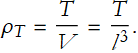
(1.33)

Apprentice Exercise 1-13: Make a table of the various units of temperature density based on °F, °C, K, in, ft, yd, mi, nm, m, and cm.

If you have done the exercises you will find that writing out the units all the time can be tiresome. It can also be tedious in calculations. We can generalize the units by writing a symbol for the quantity type being measured and then wrapping it in a square brackets. These generalized units are called dimensions. For example, length, time, mass, and temperature have dimensions, respectively, [l], [t], [m], [T].

Apprentice Exercise 1-14: Make a list of the dimensions of area, volume, mass density, and temperature density.

So, any physical quantity that is expressed in units, is called a dimensional quantity, if a quantity is not involved with units, it is a dimensionless quantity.

In any equation having dimensional quantities, each term must have the same dimensions. This is called dimensional homogeneity. You can use this property to make sure an equation is correct. Examine the dimensions of each term, if there is any difference among any term, then the equation is wrong.

It turns out that we can actually derive a formula using dimensions. How? Let’s look at an example. We will try to derive the formula for the area of a circle. We begin by writing a proposed equation for the area of a circle, , as a function of the radius of the circle, r,

(1.34)

The dimensions of both sides must be the same,

(1.35)

How do we deal with the function of radius?

(1.36)

We begin by suggesting that the function must have one or more multiples each having a coefficient and a power of the variable of the term. Such coefficients may contain constants, or other factors to allow the dimensions to become homogeneous. For now the coefficient and the power are all undefined.

(1.37)

We then write this in terms of dimensions,

(1.38)

We can then equate this with (1.9), and we will use the symbol ⇒ to represent the phrase, “implies”, or, “leads to”.

(1.39)

so both sides of this equation must have the dimensions . We do not know the dimensions of α. We do know the dimensions of r, they are also [l]. Thus we write,

(1.40)

We are left with not knowing the value of the exponent b. Since the dimensions must be the same, the power of l must be 2 in each term. There is only one such term, so we must conclude that This allows us to write the formula,

(1.40)

We now return to out examination of α, and we conclude that it has no dimensions. We cannot determine α using dimensional analysis. While we cannot get the exact form of the expression, we do know it to within a constant of proportionality, α.

Computational Lab 1: Introduction to Mathematica

Computers are electronic devices that are capable of acquiring, storing, and manipulating data in the form of binary codes. The first electronic computer of this type was made in the late 1940s to assist in calculations required for the development of the hydrogen bomb. Since then computers have become an integral part of physics. With modern computers you can collect data from instruments and experiments and store it in files, you can analyze the data, you can construct predictive models, display the data and the predictions, you can write up the results and present them in web pages, journals, and presentations.

Broadly speaking, a computer consists of a central processing unit (CPU) that controls everything, a memory unit that stores information for active use by the CPU, peripheral devices for display, long-term storage, printing, and communication with other computers, and the computer also has one or more buses for connecting all of the elements of the computer together. Most often we communicate with a computer through a keyboard and a display monitor, and we often use a mouse or a track ball.

In order to make a computer model you must be able to write out a complete list of instructions telling the computer what to do. Such a list of instructions is called an algorithm. Computers all have a language that is unique to their CPU called a machine language. Few communicate directly with the computer in machine language. Most algorithms can be converted to machine language from some other programming language through some kind of interface. Such interfaces are either active conversion as you write each instruction (this kind of language is called an interpreter), or the algorithm is written in its entirety and then converted all at once to machine language (this is called a compiler). The process of translating an algorithm into a computer language is called coding. A translated algorithm is called a computer program. Often a computer language will have a special program that contains a place where code is written, other places where information about the language is stored for reference, and there can even be tools to assist in writing your code; such a program is called a programming environment.

To operate, or run, a program the first instruction of the program is directed to the CPU and it acts on any relevant data in long-term storage. Once this is completed the results are placed in memory. The CPU is then directed to the next instruction and the process is repeated. This continues until every instruction has been completed.

Mathematica is a programming environment that uses the Wolfram Language as its computer language. The place where coding takes place is most often in a place called a notebook. The notebook is often an interpreter, though the Wolfram Language allows you to compile complicated instructions so that they run faster.

There are hundreds of computer languages and dozens of programming environments—many of them are free. This being the case, why choose Mathematica? There are many aspects that are not individually unique to Mathematica, but are collectively unique. Mathematica/Wolfram Language is platform independent (it does not depend on which operating system or CPU you use). it allows you to create programs based on algorithmic procedures (called procedural programming and this style of programming is familiar to everyone who has programmed in C, C++, Java, Python, etc.), it allows you to manipulate combinations of instructions (what we call functional programming), it allows you to rewrite instructions by applying rules (what we could call rule-based or transformational programming), and you can mix and match these kinds of programming as you like, you can create reports and finished papers (this book is written entirely in Mathematica, for example), you can import and export data, you can perform calculations that are entirely symbolic, you can perform calculations that are entirely numerical, and you can perform calculations that are both symbolic and numerical. There is no other system that has all of these capabilities that are free.

The professional/academic version of Mathematica is available from Wolfram Research and it allows you to produce code and sell it, to write technical documents (such as this book) and sell them, or to provide consulting services for pay. There is a version that is entirely in a cloud that you can log into over the Internet. There is a reduced price version for hobbyists, the caveat is that you cannot use this version for making money. There is also a version for use by students with a valid student ID. All of these versions of Mathematica are the same in terms of functionality.

When you start Mathematica it loads into memory from long-term storage. The link to the CPU is called the Mathematica Kernel. It also loads a user interface file called the Notebook Front End, or just the notebook. Multiple notebooks can be loaded at once. Notebooks can be saved into long-term storage once you name them. You can load special programs that extend the capabilities of the kernel, these are called packages.

Most of the work done in Mathematica takes place in the notebook. This front end interface easily allows you to write programs, include text, graphics, and even sound into one place. An important aspect of notebooks are the brackets that appear on the far right side, these are called cells. All instructions appear in cells. A cell encompasses a paragraph. They are the basic element of a notebook. You can copy and paste cells, you can change their format, and you can execute any instructions contained. In Windows you place the cursor anywhere in the instruction you want to execute, or you highlight the cell (by clicking on it), and then you hold down the Shift key and press Enter.

Mathematica allows you to perform each arithmetic operation and its inverse. To add two numbers, say 454 and 63, we open an Input Cell and write

To multiply two numbers, say 64 and 5155158, we can write

or we just put a space between the factors,

We can raise a number, say, 55 to a power, say 8,

we can also type 55 and then the command Ctrl 6 and then 8.

We can take the inverse of addition, subtraction by writing

The inverse of multiplication is, of course, division,

The first inverse of raising a number to a power is to take the power-order root (the surd, ()) of the exponent to get the base. Here we use the command Surd, followed by square brackets [], the square bracket is standard notation for the arguments of a built-in function.

we can also write this using a fractional power.

The second inverse of raising a number to a power is to take the base logarithm of the exponent to get the power, here the base is 55.

Let’s say we wanted to find the 9th root of our exponent,

this is an exact result, and it is very difficult to interpret it. It would be better if we could get a numerical approximation of this, we can take the previous expression and wrap an N[] around it.

Or we can write //N after the expression.

Or we can specify that we want the surd out to as many as ten decimal places

of course it doesn’t give more digits than are needed. For more details consult the built-in documentation system.

As stated above, we are not restricted to numerical calculations. When doing symbolic calculations it is a good idea to assign a name to each expression as you enter it. We will use the assignment = to assign an expression to our label. Here we invent three expressions

where the semi-colon symbol ; tells Mathematica not to display output. We can take a power

we can expand this expression.

We can take the product.

We can simplify this.

We can take the quotient

and we can factor this

We can write an equation in Mathematica by using the logical equals symbol ==. The single = tells Mathematica that we are assigning an expression to a label, the logical equality == tells us that we have an equation.

We can solve this for t.

We can specify the first solution,

or the second

You can save your work by saving the notebook in a manner consistent with your operating system.

Computational Lab 2: Units and Dimensional Analysis in Mathematica

If we want to specify that a physical quantity is being considered, where we have a numerical coefficient of a physical unit, we can do this in Mathematica by using the Quantity command, Quantity[magnitude,unit], here the magnitude is the coefficient and unit is the unit of measurement being used. For a distance of 10 m we can write,

you can use this format to encode any physical quantities.

Mathematica knows all of the measurement systems in use, all you have to do is specify the unit and it knows how to display it.

One of the uses of a Mathematica notebook is the way that you would use a page of a scratch pad. You write down the expressions you want to use, you specify the physical quantities involved, and then you can perform your calculations.

Let’s assume that you want to show a ratio between distance and the time it takes to cover that distance. We start with d1 above and say it took 10 seconds to cover it,

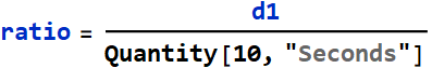
We can convert this to feet in the English system,

and we can get this as an approximation, and if you place the cursor over the result it reveals the units.

or even to Light Years (the distance light travels in a Year)

We can find the dimensions of the ratio by applying UnitDimensions

as you can see the dimensions are unchanged with other units

in either case we have dimensions [L]/[T].

Reading List

Taylor, Edwin F., and Wheeler, John Archibald, (1992), Spacetime Physics, 2nd Edition,  W. H. Freeman and Company, New York.

Peter Goldreich, Sanjoy Mahajan, and Sterl Phinney, (1999), Order-of-Magnitude Physics: Understanding the World with Dimensional Analysis, Educated Guesswork, and White Lies,  Available on the web at http://www.inference.org.uk/sanjoy/oom/ .

Lemons, Don S. (2017), A Student’s Guide to Dimensional Analysis, Cambridge University Press.

To return to the Elementary Theoretical Physics with Mathematica page click here.

To return to the main web page click here.