Creating New Functions Using Functional and Rule-Based Programming
George E. Hrabovsky
MAST
Introduction
Last time we explored how to program in the traditional procedural style. This time we will explore two paradigms that form the heart of how to use MMA/WL. The first is functional programming, programming through the use of operations on functions. The second is rule-based programming where we develop programs that take advantage of the pattern-matching and transformation systems built into MMA.
For functional programming, after a brief introduction we will explore what are called pure functions. Then we will explore how to apply functions to an existing list. Then we will discuss how to perform iterative operations. We will end our discussion of functional programming with how to compose functions and how to apply a function in operator form.
For rule-based programming, after a brief introduction, we discuss how MMA/WL handles patterns. We will discuss pattern matching. We will end with a discussion of rules.
What is Functional Programming?
Functional programming has its foundations in the development of what is called the lambda calculus founded by Alonzo Church and extended by Alan Turing, Moses Schönfinkel, and Haskell Curry in the 1920s and 1930s. In the late 1950’s John McCarthy of MIT developed the first language that used functional programming, LISP. What is a functional programming language? There is no simple definition, rather we can see what the characteristics are.
If a language allows you to pass functions as the argument for other functions, then we say that the language allows for first-class functions, another way of saying this is that functions are first-class citizens of the language.
Related to this is the existence of functions that take other functions as arguments, or they return functions as results. Such functions are called higher-order functions.
There is a kind of function whose values are the same for the same arguments. If such functions have no side-effects on the program then the function is called a pure function. This property of functions is called referential transparency.
If a function can call itself from within the function then it is called a recursive function. This replaces the tradition looping structure of the procedural program.
Functional Programming in MMA/WL
It is axiomatic that everything in MMA/WL is an expression. Many expressions are built around functions. The standard notation for functions is Head[argument(s)]. Head is that name of the function. All functions built-in to MMA/WL start with upper-case Latin letters.
If you have made an assignment it applies to the Header of a function.
![]()
![]()
In this sense, the Header itself can be thought of as an expression.
You can make a function that defines a function by using the Header as an argument.
![]()
![]()
![]()
It is this ability to treat function names as expressions that open MMA/WL to the panoply of characteristics of functional programming.
Pure Functions
There are two equivalent ways of writing pure functions in MMA/WL. The first is by writing out the Header Function.
![]()
![]()
We then apply this to a variable.
![]()
![]()
We can do the same thing using the equivalent short form.
![]()
![]()
![]()
![]()
We can apply this to functions of several arguments by numbering the short-form arguments. When using the short form we must always close the short form with the & to tell MMA/WL to stop at that point.
![]()
![]()
![]()
![]()
If we have a collection of operations we want to perform by combining functions of several arguments we use short-form for a list of all arguments.
![]()
![]()
![]()
![]()
![]()
![]()
If we have a list of arguments and we want to ignore the first one, we use the short form of the list of arguments except the first n, ##n, where n tells MMA/WL where to start the list of arguments.
![]()
![]()
![]()
![]()
Applying Functions to Lists
If we want to apply a function to a list we use Apply.
![]()
![]()
We can also use the short form.
![]()
![]()
Here is an example
![]()
![]()
If we want to apply a function to every element in a list we use the Map command.
![]()
![]()
We can also use the short form the we introduced in lesson 2.
![]()
![]()
For a more concrete example.
![]()
![]()
We can also use this to apply a function to another list of functions.
![]()
![]()
![]()
![]()
Say we have a matrix.
![]()
![]()
We can apply Map to the individual elements of the matrix.
![]()
![]()
There is another type of command that applies the function to every level of the matrix.
![]()
![]()
There are three levels of the matrix to which the function can be applied to: the whole matrix, each row, and then each element of the row. We can use the short form of this, too.
![]()
![]()
We can get a list of the levels and their positions.
![]()
![]()
We can see this in the row of the matrix, too.
![]()
![]()
We can also apply this to all levels.
![]()
![]()
We can map a function to a part of an expression or list. Here we map a function to the third part of a list.
![]()
![]()
Here we have a new matrix.
![]()
![]()
The first row is part 1, the second part 2, both rows have three parts in their own right. Here we map a function to the first part of the first row, and the second part of the second row.
![]()
![]()
While Map produces a new expression, we might want to apply a function of a list without creating a new expression. To do this we can use the Scan command.
![]()
![]()
![]()
![]()
We can also apply a function to parts of an expression.
![]()
![]()
![]()
![]()
![]()
Iterations with Functions
As stated earlier in functional programming we do not use looping structures, we use recursion. In MMA/WL the Nest command applies a function recursively a number of times on an expression. We write Nest[function,expression,number of recursive steps]. We can make up an abstract example.
![]()
![]()
For example we can see how to recursively apply a square root to the number 100 five times.
![]()
![]()
We can write this as a pure function.
![]()
![]()
If we want to see each intermediate value of the recursion process we use the NestList command.
![]()
![]()
For the example we developed, we get this result.
![]()
![]()
Sometimes we want to recursively work with a function until a result no longer changes. We do this with the FixedPoint function. We write FixedPoint[function, starting point]. This example comes from the Tutorial Functional Operations included in the documentation. The goal will be to apply Newton’s approximation of the square root of three, we begin with a single step.
![]()
We choose a starting point of x=1.
![]()
![]()
We can see how many recursive steps are required by using the FixedPointList command.
![]()
![]()
We can also apply a function recursively until a test fails. We write NestWhile[function,starting value,test], here is an example. We devise a function to divide a number by some divisor, say 2.
![]()
![]()
![]()
We can see the intermediate values.
![]()
![]()
Say we want to apply a function recursively for a fixed argument, and a second argument is from a list.
![]()
![]()
We can see each recursive step.
![]()
![]()
Another Notation for Functions
There is an important way of writing some functions. For example, here we take the derivative of the function f with respect to the variable x.
![]()
![]()
This is the wrong answer, we need to write the function correctly.
![]()
![]()
Another way to write this is with the derivative operator.
![]()
![]()
Or we can use a new way of writing it. Command [function head] [variable]. For example we can write the derivative.
![]()
![]()
Note that this last allows for abstract function place holders to be used. We can do this without a variable.
![]()
![]()
So this form of function can be very useful. It is not implemented for every function. Check the documentation to see if it is available for the function you want to use.
Functional Composition and Operators
In set theory, and thus all of mathematics—using set theory as its foundational language—there is an operation where one function is allowed to operate on another function. This is called a composition. If the function f is allowed to operate on the function g(x), the composition is written f◦g or f(g(x)). Here is how we compose functions in MMA/WL.
![]()
![]()
We can also use the short form.
![]()
![]()
We can reverse the direction of the composition.
![]()
![]()
Here is its short form.
![]()
![]()
We can compose the inverse functions.
![]()
![]()
Using the Identity command returns the suitable identity result.
![]()
![]()
Through performs the same task as apply, except for the Heads.
![]()
![]()
This example is taken from the documentation. If we define a differential operator.
![]()
![]()
Now we use Through to apply the operator to a sine function.
![]()
![]()
Here we construct a table of natural logarithms
![]()
| 0. | Indeterminate |
| 1. | 0. |
| 2. | 0.693147 |
| 3. | 1.09861 |
| 4. | 1.38629 |
| 5. | 1.60944 |
| 6. | 1.79176 |
| 7. | 1.94591 |
| 8. | 2.07944 |
| 9. | 2.19722 |
| 10. | 2.30259 |
If we want a function to operate on another function we can write Operate[function a,function b[arguments]].
![]()
![]()
Here is an example.
![]()
Operate defaults to the level 1 specification, this is the head. We can choose to specify the level.
![]()
We can apply Operate recursively.
![]()
The process of transforming a collection of sublists into a single list is called flattening the list. We write Flatten[list]. Here we have a complicated list of sublists, taken from the documentation.
![]()
![]()
![]()
![]()
Here we flatten only at level 1.
![]()
![]()
We can use Flatten to work with heads
![]()
![]()
We can choose which Head to flatten.
![]()
![]()
![]()
![]()
Sometimes we want to flatten elements at only specific locations in a list. We use FlattenAt[list,element number].
![]()
![]()
What is Rule-Based Programming?
Rule-based programming is based on formal logic. We establish a set of rules, based on patterns and pattern matching. The rules transform the results in ways that we choose. The programs are built up out of the transformation rules.
The history of rue-based programming extends back to the 1960s and is a bit murky. The first really successful language came out in 1972 when Alan Colmerauer collaborated with Philippe Roussel (using prior work done by Robert Kowalski) in Marseilles, France. This resulted in a language called Prolog.
Patterns
When we want MMA/WL to know that something is a pattern we want it to remember for the line of code being made, we use a blank. Pattern_ tells MMA/WL that Pattern needs to be looked at. In function a pattern in the argument is applied to the body of the function. Here is a function to find the prime. We only want integers as input.
![]()
![]()
![]()
The short form x_ is the same as another form x:_.
If we want MMA/WL to look for a pattern with one or more elements we use the double underscore. This represents a BlankSequence. The label represents the name of the sequence in the body of pattern.
![]()
![]()
![]()
![]()
![]()
![]()
Here, again, x__ is the same as x:__.
If we want MMA/WL to look for a pattern with zero or more elements we use the triple underscore. We call this a BlankNullSequence
![]()
![]()
![]()
When we want to specify different options for patterns as use a vertical line, |, to separate them, this is the short form of the command Alternatives.
![]()
![]()
![]()
![]()
![]()
![]()
![]()
![]()
![]()
![]()
If we have a sequence of arguments, but we don’t care what order we input them we can use OrderlessPatternSequence[pattern list]. This example is taken from the documentation.
![]()
![]()
![]()
![]()
![]()
![]()
![]()
We can do this for all argument of a function by using the SetAttributes command and the Orderless command. This example is taken from the documentation.
![]()
![]()
![]()
There are times when we want a default argument in a function. Default[function head] is the command to use. In this state the function is written with an argument pattern function[arg_.] where _. is a pattern that can be ignored.
![]()
![]()
![]()
![]()
![]()
![]()
![]()
![]()
If you want to look up all of the attributes of a command or symbol use the Attributes[symbol].
![]()
![]()
Pattern Matching
If we have a list, and we want to get a sublist of all elements that match a pattern we use Cases[list,pattern]. For example, if we want to know what elements of a list that are Integers, we might have something like this.
![]()
![]()
If we want to know where a matched element is in an expression, we use Position[expression,pattern].
![]()
![]()
![]()
![]()
If we want to know how many elements of a list match a pattern we use Count[list,pattern]. This example is taken from the documentation.
![]()
![]()
We can also apply this to associations.
![]()
![]()
Note that this only counted those cases that matched the pattern in level 1.
![]()
![]()
If we want to remove all elements from a list that matches a pattern we use DeleteCases[list,pattern]. These examples are taken from the documentation.
![]()
![]()
Or in operator form.
![]()
![]()
If we have a pattern matching problem and we want the expression unevaluated during it, we use the HoldPattern[expression] command.
![]()
![]()
![]()
![]()
Rules
A Rule is a statement where lhs is transformed into the rhs by the relation of an arrow lhs→rhs. We can make this a replacement rule by ending an expression with the ReplaceAll symbol /. as we see here.
![]()
![]()
If we want a different result each time a replacement rule is evaluated we use the RuleDelayed symbol. This is :> . Here is an example from the documentation.
![]()
![]()
If we want to perform a transformation recursively until the result no longer changes we use ReplaceRepeated, //., here is an example from the documentation. MMA/WL does not apply the properties of the logarithm.
![]()
Here is what we get when we use the ReplaceAll command.
![]()
![]()
Here is what happens when we use ReplaceRepeated.
![]()
![]()
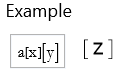
If we need to use an input exactly in a rule or pattern we use the Verbatim[expression] command. This example is taken from the documentation. We begin with a delayed rule to take the square of an expression.
![]()
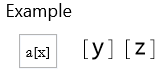
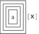
We can apply this to an expression
![]()
![]()
If we want to make this work only for specific number types we can write.
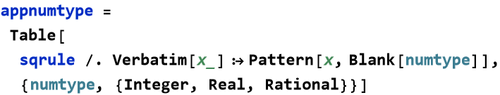
![]()
![]()
![]()
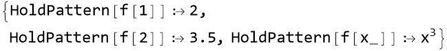
Values assigned directly to a function are called downvalues. We can see a list of these by using the DownValue[function head] command.
![]()
![]()
We can use the language here to write our own downvalues.
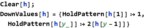
![]()
We can use the Definition command to see how a symbol is defined.
![]()
|
![]()
![]()
Values assigned directly to composed functions are called upvalues. We can use UpValues[function head] to find these rules. Here is an example from the documentation.
![]()
![]()
![]()
![]()