Introduction to Mathematica

George E. Hrabovsky

MAST

Introduction

Welcome to this course on Mathematica. The purpose of this course is to provide a comprehensive introduction to Mathematica (MMA) and its underlying programming language, the Wolfram Language (WL). The course consists of six lessons. This lesson provides a non-programming-oriented introduction to Mathematica. The second lesson begins the programming orientation by showing how you can use traditional procedural-style programming to invent new functions in WL. The third lesson will show how to use functional and rule-based programming to invent new functions. The fourth lesson will show how to use scoping construction (local variable structures) to invent new functions, and to create interactive functions. The fifth lesson will discuss the notion of best practices in developing new functions. The final lesson will introduce notions of debugging and testing, code optimization, and how to make larger systems, including writing your own packages.

This lesson will introduce MMA and WL from the perspective of a new user. We begin by discussing why MMA is revolutionary and why you should use it. We will also discuss some myths that have grown up around MMA and WL. We will discuss the origin and evolution of MMA from its beginnings to the present day. We will discuss the structure of MMA and why it is important to understand it. We will then turn to a lengthy discussion of how to use MMA for performing calculations. We then turn to the issue of using MMA for visualization of function behavior. We end with a discussion of how to get more information within MMA.

Computers are electronic devices that are capable of acquiring, storing, and manipulating data in the form of binary codes. The first electronic computer of this type was made in the mid to late 1940s to assist in calculations required for the development of the hydrogen bomb. Since then, computers have become an integral part of daily life. With modern computers you can collect data from instruments and experiments and store it in files, you can analyze the data, you can construct predictive models, display the data and the predictions, you can write up the results and present them in web pages, journals, and live presentations.

Broadly speaking, a computer consists of a central processing unit (CPU) that controls everything, a memory unit that stores information for active use by the CPU, peripheral devices for display, long-term storage, printing, and communication with other computers, and the computer also has one or more buses for connecting all of the elements of the computer together. Most often we communicate with a computer through a keyboard and a display monitor, and we often use a mouse or a track ball.

In order to make a computer model you must be able to write out a complete list of instructions telling the computer what to do. Such a list of instructions is called an algorithm. Computers all have a language that is unique to their CPU called a machine language. Few people communicate directly with the computer in machine language. Most algorithms can be converted to machine language from some other programming language through some kind of interface. Such interfaces use either active conversion as you write each instruction (this kind of language interface is called an interpreter), or the algorithm is written in its entirety and then converted all at once to machine language (this is called a compiler). The process of translating an algorithm into a computer language is called coding. A translated algorithm is called a computer code or program. Often a computer language will have a special program that contains a place where code is written, other places where information about the language is stored for reference, and there can even be tools to assist in writing your code; such a program is called a programming environment.

To operate, or run, a program the first instruction of the program is directed from long-term storage to the CPU and it acts on any relevant data that is kept in long-term storage for this purpose. Once this is completed the results are placed in memory. The CPU is then directed to the next instruction and the process is repeated. This continues until every instruction has been completed.

Mathematica is a programming environment that uses the Wolfram Language as its computer language. The place where coding takes place is most often in a place called a notebook. The notebook is often an interpreter, though WL has a compiler that is becoming integrated into more and more functions with every new version release and it allows you to compile complicated instructions so that they run faster. Thus MMA can be thought of as a hybrid interpreter/compiler.

There are hundreds of computer languages and dozens of programming environments—many of them are free. This being the case, why choose Mathematica? MMA has many useful aspects that are not individually unique to it, but are collectively unique. MMA/WL is platform independent (it does not depend on which operating system or CPU you use). it allows you to create programs based on algorithmic procedures (called procedural programming and this style of programming is familiar to everyone who has programmed in C, C++, Java, Python, etc.), WL also allows you to manipulate combinations of instructions (what we call functional programming), it allows you to rewrite instructions by applying rules (what we could call rule-based or transformational programming), and you can mix and match these kinds of programming as you like, you can create reports and finished papers (this lesson is written entirely in Mathematica, for example), you can import and export data, you can perform calculations that are entirely symbolic, you can perform calculations that are entirely numerical, and you can perform calculations that are both symbolic and numerical. There is no other system that has all of these capabilities that are free.

The professional/academic version of Mathematica is available from Wolfram Research and it allows you to produce code and sell it, to write technical documents (such as this lesson) and sell them, or to provide consulting services for pay. There is a version that is entirely in a cloud that you can log into over the Internet. There is a reduced price version for hobbyists, the caveat is that you cannot use this version for making money. There is also a version for use by students with a valid student ID. All of these versions of Mathematica are the same in terms of functionality.

There are some of repeated statements made about MMA/WL that are not true. Many people choose not to use MMA because it is slow compared to some other language. It might be true that optimized code in a special language might be a few percent faster than MMA, but there are two things that need to be pointed out. If you convert directly from, say, a procedural language to procedural code in MMA it is not the most efficient use of MMA. It is better to choose what parts of MMA are best for the algorithm you want to code (perhaps even changing the algorithm). The other thing to consider is development time, MMA requires only a fraction of the time to code as other languages. If you optimize the implementation of an algorithm in MMA/WL it will run competitively.

Another complaint is that MMA is a black box, where you have no idea what is going on once you start using a built-in function. It is true that some functions in WL or MMA are so complicated and huge that the specific method being used is not easy to follow. There is a continual struggle to document functions and methods that often lags behind development. On the other hand you are not restricted to use built-in functions. If you are uncertain about how something is being done, write your own. Compare it with the built-in function. The purpose of this course is to allow you to extend the capabilities of MMA to include things that you want.

Another complaint is that MMA/WL can only handle small projects on a desktop computer. That is sheer nonsense. Wolfram|Alpha is an online interactive system maintained on a large cluster of computers accessible to anyone over the Internet and consists of millions of lines of MMA/WL code.

Some Historical Context

Mathematica was developed, originally, by Stephen Wolfram. His story is very interesting in its own right. Mathematica was not his first foray into the development of software.

SMP (Symbolic Manipulation Program) was pretty revolutionary for its time, it was developed by Chris Cole and Stephen Wolfram in 1981 while they were at Caltech. It was one of a few programs called computer algebra systems (CAS), they allowed symbolic programming. Other contemporary CAS programs were Reduce and Macsyma.

When Wolfram left Caltech he was unable to take SMP with him, as it was being sold by a different company. Wolfram, along with other developers produced the first commercial version of MMA in 1988 where it had approximately 500 functions. Each new version added new functions where the newest version has more than 6000 built-in functions. Of course, it has always had a programming language that in 2013 was officially named The Wolfram Language (WL). So, if it doesn’t do something you want it to do, you can program a new function or even a large software system.

The Structure of Mathematica

When you start Mathematica it loads into memory from long-term storage. The link to the CPU is called the Mathematica Kernel. It also loads a user interface file called the Notebook Front End, or just the notebook. Multiple notebooks can be loaded at once. Notebooks can be saved into long-term storage once you name them. You can load special programs that extend the capabilities of the kernel, these are called packages.

Most of the work done in Mathematica takes place in the notebook. This front end interface easily allows you to write programs, include text, graphics, and even sound into one place. An important aspect of notebooks are the brackets that appear on the far right side, these are called cells. All instructions appear in cells. A cell encompasses a paragraph. They are the basic element of a notebook. You can copy and paste cells, you can change their format, and you can execute any instructions contained in such a cell. In Windows you place the cursor anywhere in the instruction you want to execute, or you highlight the cell (by clicking on it), and then you hold down the Shift key and press Enter.

If you have a multiprocessor computer, then you can have a number of kernels running in parallel, one on each of a number of processors (usually half the number of processors you have on your computer). If you have a network of computers, and each computer has MMA, then you can connect them over a local-area network (LAN)  by using the built-in Lightweight Grid. This allows you to have different processes operating on multiple cores or multiple computers.

The fundamental object that is placed in active memory is called an expression. Everything you work on in a cell is an expression, whether it is a calculation, a paragraph of text, an image, a sound file, a video, or any combination. MMA/WL has a sophisticated system for interpreting expressions. Say we have the expression a+b. This is an expression made up of three sub-objects that we can call tokens. There are two symbolic tokens, a and b, and one operator token +. MMA/WL looks at the expression and see the operator first in the form of a header, Plus, then the symbols, so it sees Plus[a,b]. Simple expressions can be used to build more complicated expressions.

New functions can be created in notebooks. Sometimes, especially with large collections of functions we might place them all into a special notebook that we call a package. A package is stored in a folder called AddOns and as you might expect they are loaded to add new functionality to MMA/WL.

Using Mathematica for Calculation

Mathematica allows you to perform each arithmetic operation and its inverse. To add two numbers, say 454 and 63, we open an Input Cell and write

To multiply two numbers, say 64 and 5155158, we can write

or we just put a space between the factors,

Note that MMA fills in a multiplication symbol when applying the space to numbers.

We can raise a number, say, 55 to a power, say 8,

we can also type 55 and then the command Ctrl 6 and then 8.

We can take the inverse of addition, subtraction by writing

The inverse of multiplication is, of course, division,

The first inverse of raising a number to a power is to take the power-order root (the surd) of the exponent to get the base. Here we use the command Surd, followed by square brackets [], the square bracket is standard notation for the arguments of a built-in function.

we can also write this using a fractional power.

The second inverse of raising a number to a power is to take the base logarithm of the exponent to get the power, here the base is 55.

Let’s say we wanted to find the 9th root of our exponent,

this is an exact result, and it is very difficult to interpret it. It would be better if we could get a numerical approximation of this, we can take the previous expression and wrap an N[] around it to get a floating-point approximation.

Or we can write //N after the expression.

Or we can specify that we want the surd out to as many as ten decimal places

of course it doesn’t give more digits than are needed.

As stated above, we are not restricted to numerical calculations. When doing symbolic calculations it is a good idea to assign a name to each expression as you enter it. We will use the immediate assignment symbol = to assign an expression to our label. Here we invent three expressions

where the semi-colon symbol ; tells Mathematica not to display output. We can take a power

we can expand this expression.

We can take the product.

We can simplify this.

We can take the quotient

and we can factor this

We can write an equation in Mathematica by using the logical equals symbol ==. The single = tells Mathematica that we are assigning an expression to a label, the logical equality == tells us that we have an equation.

We can solve this for t.

We can specify the first solution using the symbol for the element of a list,

or the second

If we want to specify that a physical quantity is being considered, where we have a numerical coefficient of a physical unit, we can do this in Mathematica by using the Quantity command, Quantity[magnitude,unit], here the magnitude is the coefficient and unit is the unit of measurement being used. For a distance of 10 m we can write,

you can use this format to encode any physical quantities.

Mathematica knows all of the measurement systems in use, all you have to do is specify the unit and it knows how to display it.

Let’s assume that you want to show a ratio between distance and the time it takes to cover that distance. We start with d1 above and say it took 10 seconds to cover it,

We can convert this to feet in the English system,

and we can get this as a decimal approximation, and if you place the cursor over the result it reveals the units.

or even to Light Years (the distance light travels in a Year)

We can find the dimensions of the ratio by applying UnitDimensions

as you can see the dimensions are unchanged with other units

in either case we have dimensions [L]/[T].

There are two powerful commands for simplifying expressions. The act of simplification is a set of transformations that result in the most reduced form of the expression. The first is Simplify[expression]. Here we have a simplification of a polynomial.

Note that the order is reversed from the way most of us would write it. We can use the // to put a command at the end of the instruction. We can use the instruction TraditionalForm to write the answer in a nice font and in a way that matches how we might write on a note pad.

Here we have a rational expression.

Sometimes we will need to make assumptions clear before getting the answer we want. Here is an example.

While this is true, it is not very useful. We note our assumption that x∈R,

That’s better.

We can also use the Assuming command first,

FullSimplify can be used if Simplify is not effective. Warning FullSimplify takes more time.

Expand allows you to expand products and integer powers. For example.

PowerExpand allows you to expand all products of powers and powers.

We can use ExpandAll when we have a combination of sums and powers.

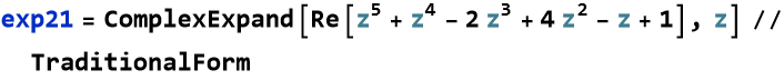
ComplexExpand allows us to expand complex expressions. Here we see the results for a complex polynomial.

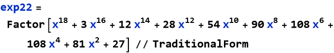
Factor allows us to factor a polynomial.

Collect[expression,form] collects terms of powers that match the form specified.

We can simplify this,

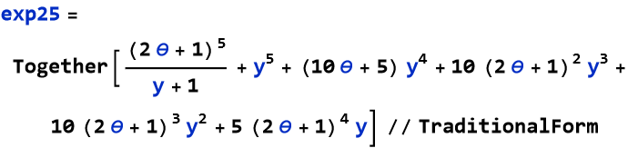
Together places the terms into a sum over a common denominator

Refine allows us to convert a symbolic expression to one where a numerical factor would be included, returning to an example from above we see

Distribute allows us to apply the distributive law over an operator, in this case multiplication,

Distribute does not perform the addition in the correct order, so the product disappears.

To do it correctly we can use the command Unevaluated around the product, this allows the product to be done in the correct order.

Apart makes a rational expression into a sum of minimal denominators,

Here are some examples of trigonometric expressions, these apply relevant trigonometric identities.

Simplify does this automatically.

PowerExpand does not,

instead we use  TrigExpand

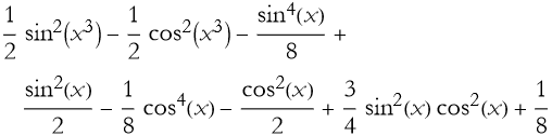
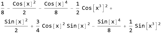
TrigReduce should reverse the expansion.

Why did it fail? TraditionalForm is the problem. How do we get expressions to work correctly and display the way we want them to? Wrap the TraditionalForm around the expression instead of applying it at the end.

this does not change the expression,

Mathematica can symbolically solve equations, note that the result is in the form of a transformation.

We can remove a level of brackets by specifying the first solution.

Or we can tell Mathematica to display the solution and transform the symbol for x according to the solved equation.

We can reproduce the quadratic formulas. There are two solutions, so the result is a list of two solutions. We can specify the first element of the list.

Here is the second element of the list of solutions.

Mathematica can solve systems of equations, too.

Or we can perform a real approximation of these exact results,

Using Mathematica for Visualization

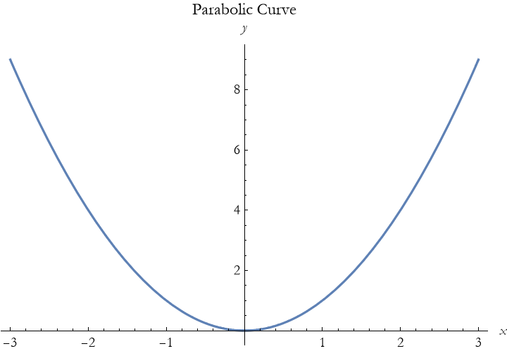
The plot command plots an expression for an independent variable over a specified range of values.

We can easily make this plot useful to all viewers by labeling the axes with nicely formatted labels, and providing a label for the plot itself. Show allows us to combine many graphics command into a single unit. GrayLevel->0 is the value for black.

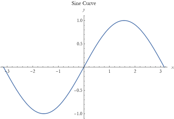
Here we show how Mathematica handles a trigonometric function.

Using Mathematica as a Scratch Pad

One of the uses of a Mathematica notebook is the way that you would use a page of a scratch pad. You write down the expressions you want to use, you specify the physical quantities involved, and then you can perform your calculations.

Most of you have done this with a sheet of paper, where you start by writing out what you know and then working the problem through successive calculations, notes, and diagrams.

You can easily use MMA notebooks as scratch pads in the same way.

Using the Mathematica Help System

You can look things up in the documentation systems. If you note the Help Menu at the top of the notebook, you can access the system there. When you choose the Help Menu you then choose Wolfram Documentation and a user interface window opens up.

If you know what you are looking for you can type it into the search bar at the top of the screen.

You might not know what you are looking for. There are four main parts of the interface to find what you want. First, there are a series of colored blocks that you can click on. Then there are a number of gray buttons entitled workflows. Another set of gray buttons called resources. Finally there are four text-based links at the bottom.

Examining the colored blocks you will note four colors. The orange blocks are six aspects of the system itself. The yellow blocks represent types of expressions. The green blocks represent types of applications. The blue blocks represent deliverables.

The six orange blocks are Core Language and Structure, dealing with fundamental aspects of the Wolfram Language and how to program in it. Data Manipulation and Analysis are a collection of aspects relating to collections of data that you as the user provide. Visualization and Graphics explore how to represent functions and data. Machine Learning is where you can look up functions allowing you to construct machine learning capabilities, that is to teach the machine to do a number of tasks in an almost autonomous way. Symbolic and Numeric Computation covers using WL to perform mathematical operations. Higher Mathematical Computation deals with advanced  mathematics.

The six yellow blocks begins with Strings and Text, these are functions that allow you to process strings and text in programming. Graphs and Networks allow you to explore such objects a directed graphs and the subject of both graph theory and its related network theory. Images explores the MMA/WL ability to analyze and enhance images. Geometry explores geometrical objects.  Sound and Video allow you to analyze and enhance audio files and video files. Knowledge Representation and Natural Language explore how MMA/WL uses knowledge-type structures in programming.

The six green application blocks begin with Time-Related Computation, exploring time-based dynamical systems. The remaining green blocks have collections of functions allowing you to explore curated data and applications of a specific nature: Geographic, Scientific and Medical, Engineering, Financial, and Social/Cultural/Linguistic.

The six blue deliverable blocks begin with Notebook Documents and Presentation that collect functions allowing you to control various aspects of notebooks that you can program to create documents, web pages, reports, and slide shows. User Interface Construction explore functions allowing you to create graphic user interfaces (GUIs) for any occasion. System Operation and Setup are functions that allow you to tailor your use of MMA/WL. External Interface and Connections are functions related to networking and how to share information. Cloud and Deployment  are functions related to cloud-type environments. Recent Features explore new functions from the most recent versions.

There are twelve workflow blocks. What is a workflow? A workflow is a repeatable pattern of activity to provide some service or to process some kind of information. You can think of it as an algorithm connecting materials, services, and information through a sequence of operations. In MMA/WL the workflow buttons provide suggestions on how to proceed with specific types of workflows.

The six Resource blocks provide resources to support you continuing development as a MMA/WL user/programmer. One homework assignment will be to work through one, or both, of the fast introductions. The Intro Book and Course connects you via the Internet to an online version of Stephen Wolfram’s introductory book in programming in the WL. Archives and repositories connect you to one of several online collections maintained by Wolfram Research. The function repository is very useful as it contains user-developed functions not implemented into MMA/WL but are useful (in fact you can create your own functions and share them here for other users). Resources for Software Developers are a collection of free tools for developing software (including free Wolfram Engine for developers), there are also other development environments that you can download. There are other Wolfram Language products than MMA. Then there are a number of educational resources through Wolfram U.

Palettes are arrays of buttons that produce specific output can be found in the Palettes menu. Many of these are useful and you can, or course, create your own.

If you are in a notebook and you want to find out about a function you are using, you can type a question mark and then the function name. For example,

I will end with a warning. The  documentation in MMA consists of literally thousands of pages of free resources. It is very easy to get sucked in while searching and spend hours poking around. It is usually fun and you almost always find new things. Beware of getting sucked down these rabbit holes, it happens to me all the time!