An Introduction to Mathematica
George E. Hrabovsky
MAST
What We Will Cover
Here is the agenda of this talk.
What Is Mathematica?
What is a Computer Algebra System?
What is the Structure of Mathematica?
What are the core principles of Mathematica?
How Do We Use Mathematica?
The Documentation System
Mathematica as a Scratchpad
Mathematica as a Discovery Tool
Mathematica as a Programming Environment
Mathematica as a Computational Lab
Mathematica as a Word Processor
Mathematica as a Classroom
Where Can I Get Mathematica?
What Now?
Free-form workshop setting to demonstrate how to do things.
What Is Mathematica?
Mathematica is a computational environment allowing for many modes of operation:
You can use its built-in capabilities as a Computer Algebra System (CAS) to do symbolic mathematical work.
You can use its built-in capabilities to perform numerical mathematical work.
You can use it as a scratch pad for mathematical work.
You can use it for data analysis and visualization.
You can use it for image and audio processing.
It is a fully capable programming language allowing you to use and mix programming paradigms at will.
You can use it to create and maintain documents and slide shows.
We will see how many of these capabilities work.
What is a Computer Algebra System (CAS)?
This is a now, mostly, outdated term to describe systems that allow you to perform symbolic mathematical operations on a computer instead of the tradition numerical operations. I consider it outdated because niether of the two principle systems (Mathematica and Maple) are strictly algebra systems, as they both have very capable numerical and general programming capabilities.
The first CAS I know of was called MathLab and came out in 1964. It brought about what can be considered the first generation of CAS. These are exclusively written in, and require the use of, the programming language LISP.
Reduce came out in 1968, it is now in the public domain. Reduce is also a first-generation system—it is written in, and requires, LISP. It is freely available form the website: http://www.reduce-algebra.com/ .
Then Macsyma was developed,in 1969. This had an interesting development path. Macsyma was sold commercially for a while, and is now defunct. MIT had a version of it under the DOE, called Maxima, which entered the public domain. This is now available at the website: http://maxima.sourceforge.net/ .
Scratchpad was the next first-generation system and it came out in 1974,. This is was a remarkable system that later became Axiom,. Axiom is now terribly out of date, at least in terms of its interface, and is available at the web site: http://axiom.axiom-developer.org/ .
MuMath, which later became Derive, came into being in 1979, and was the last of the first-generation systems developed in LISP. Derive had an interesting life. Starting out as a reduced-strength CAS for students, it saw life in certain powerful hand-held calculators.
Maple is a second-generation system written in C and C++ and first arrived in 1983 from Waterloo Software (now owned by Cybernet Systems Group). It is now a fully capable environment for programming and scientific discovery.
MuPAD came out in 1992 and is available only as a MATLAB add-on. I consider this to be extremely expensive, since you need MATLAB and then MuPAD.
Mathematica came out in 1988, also written in C/C++, is the most popular of the general CAS. It began around 1981 when Stephen Wolfram wrote the SMP CAS while at CalTech.
What is the Structure of Mathematica?
The Kernel(s)
This is the part that does all of the work. It can be thought of as an internal engine. It interprets all commands, processes all requests, and produces all output. The computational engine is called the Wolfram Language.
The Mathematica Notebook
This is the most common interface with the kernel. You type in the input and the formatted output is displayed. It is a file that allows you to record your sessions and produce high-quality typesetting. All input and output are in the form of cells marked by brackets on the right hand side of the notebook
What are the Core Principles of Using Mathematica?
Everything in Mathematica takes place in a cell. Cells are bounded on the right by the square brackets you see. Cells allow you to perform operations on whatever is within the cell. You can copy, cut, delete, and paste cells. As we go we will see other operations we can perform on cells, too.
Everything within a Mathematica cell is an expression. It can be a number, a string of text, a paragraph, an equation, a command, a photograph, a piece of music, a program, or a database—all are examples of expressions in Mathematica. There are numerous ways to manipulate expressions, and we will get around to exploring them.
An expression that accepts input and produces output is called a function. In Mathematica there are two aspects of functions that are important. First, all Mathematica functions begin with an upper-case letter. Second, after the function label, called the Head in Mathematica-ese, are enclosing square brackets [ ], where you place the expression that the function is to act on, called the Argument of the function.
How Do We Use Mathematica?
We can open a cell by placing the cursor at a new line and just start typing.
You can also put the cursor at a new line and click on the tab. In presntation mode the tab does not appear.
You can change the form of a cell by highlighting the bracket, and then choosing the cell type you want. Make sure the formatting toolbar is active.
Now we open a cell. Then we choose the format Input. Then we type an expression. We can tell Mathematica to evaluation by holding down the [SHIFT] key and then typing [ENTER]. On a Mac this sequence is different.
Notice that we now know about text cells, input cells, and output cells.
Mathematica, not suprisingly, understands arithmetic. It can add,
![]()
![]()
it can multiply,,
![]()
![]()
it can raise a number to a power
![]()

It also has functions for each of these operations.
![]()
![]()
![]()
![]()
![]()

Mathematica knows about the inverse operations, too.
![]()
![]()
![]()
![]()
![]()
![]()
We can get the numerical approximation of this by adding a function on the end using //, then naming the function, in this case N.
![]()
![]()
![]()
![]()
Assume we have the power
![]()
![]()
There are two inverses, the 6th root and the base 12 logarithm.
![]()
![]()
![]()
![]()
![]()
![]()
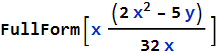
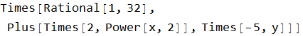
We can get a clue about how Mathematica is evaluating a calculation by using the command FullForm[ ]
We can get a graphical representation of this using TreeForm[ ]
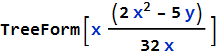

Note that when you mouse over the squares, at least in Mathematica or the CDF reader (we will discuss this later on).
Mathematica can deal with units of measurement in a primitive way. For example, if we want to determine the distance traveled at some speed,
![]()
![]()
Note that Mathematica handles all simplifications.
Mathematica can deal explicitly with units by using the Quantity[ ] command.

![]()
This generates a warning, to suppress it we aply the Quiet command.
We can then convert between units using the UnitConvert[ ] function
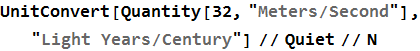
![]()
In Mathematica there are two kinds of assignments. Both types allow you to label an expression.and call that expression whenever you use that label.
An immediate assignment uses the = symbol and it immediately applies the expression to the label.
![]()
![]()
![]()
![]()
A delayed assignment holds the value of the expression as unevaluated until it is requested.
![]()
![]()
![]()
![]()
![]()
![]()
![]()
![]()
![]()
![]()
![]()
The delayed versions executes the command afresh every time you use it.
We can refer to the previouis output using the %% symbol.
![]()
![]()
Note that every output cell has a number associated with it. We can refer to a previous result by using the %number symbol.
![]()
![]()
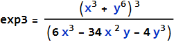
A more sophisticated, and easier to understand, method of assignment is to label each expression, then refer to it through that assignment.
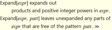
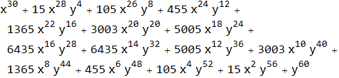
Mathematica understands algebra. Here we use the Expand[ ] function.
![]()

We can also Factor[ ]
![]()
![]()
![]()
We can pull out parts of an expression using Coefficient[ ], Exponent[ ], Part[ ], Numerator[ ], and Denominator[ ]
![]()
![]()
![]()
![]()
![]()
![]()
![]()
![]()
![]()
![]()
![]()
![]()
![]()
![]()
We can rearrange formulas by collecting in terms of the powers of a specified variable using Collect[ ]
![]()
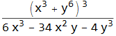
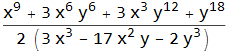
We can gather a sum over a common denominator using Together[ ]
![]()

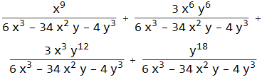
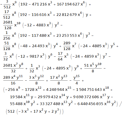
We can separate an expression into more terms using Apart[ ]
![]()
We can use the function Cancel[ ] to remove common factors between a numerator and denominator.
![]()
It is rare when you have only a single value for a variable. Mathematica allows you to manipulate lists of expressions. You can create them manually using curly brackets.
![]()
![]()
When we want to use a symbol later, we can clear its assignmernt if we decide it is not important.
![]()
For example, we can assign the components of a vector,
![]()
![]()
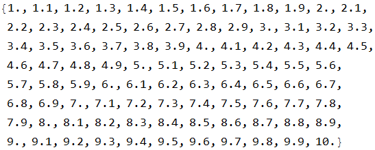
We can also use Range[ ]
![]()
![]()
![]()
You can create lists using a table, Table[ ]
![]()
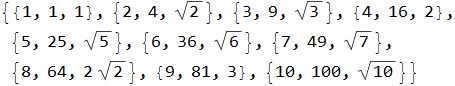
![]()
| 1 | 1 | 1 |
| 2 | 4 | |
| 3 | 9 | |
| 4 | 16 | 2 |
| 5 | 25 | |
| 6 | 36 | |
| 7 | 49 | |
| 8 | 64 | |
| 9 | 81 | 3 |
| 10 | 100 |
![]()
| 1 |
| 2 t |
![]()
![]()
Table is a very powerful programming tool. Learn to use it!
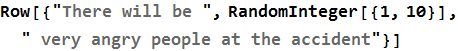
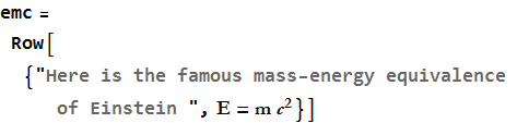
We can use Row[ ] to create structured output.
![]()
![]()
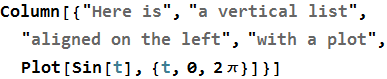
We can use Column[ ] too,
| Here is |
| a vertical list |
| aligned on the left |
| with a plot |
 |
If we have a formula, we can use Plot[ ] to represent its curve graphically.
![]()
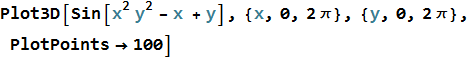
For functions of two variables, we can use Plot3D[ ]
We can also use ContourPlot[ ]
![]()
and DensityPlot[ ]
![]()
The Documentation System
Of course, it is impossible to cover all of the functions in Mathematica in a comprehensive way. Each version of Mathematica over the last three years have produced more functions than existed in the original version. Get to know the documentation system. You access it through the Help Menu. There are thousands of pages of very useful information.
![]()
Mathematica as a Scratchpad
The easiest way to use Mathematica is a scratchpad. You use it just like you would a piece of paper. We will do this when we get to the workshop section of this presentation.
Mathematica as a Discovery Tool
If you are messing around, or you don’t know where to start you can always try free-form input. You can choose this from the tab,
Or you can hold down the [CTRL] key and then type =
Notice that the free-form input is transformed into its Wolfram Language equivalent. For example, if we type in, “derivative of sine of x”
![]()
You can also, assuming you are connected to the Internet, launch a WolframAlpha session.
![]()
Mathematica as a Programming Environment
Mathematica is also a fully-functional programming environment within the notebook front end.
The simplest type of program is to create your own function
![]()
![]()
![]()
Note that we used an underscore in the function name, this is a place holder and tells Mathematica to replace the underscored lable with whatever you type in in the function command.
We can separate the names of local variables from global variables using Module[ ]
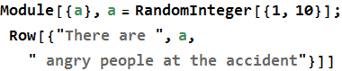
![]()
You can separate local values from global values using the Block[ ] function. For example, you can use Block[ ] to use a variable name used elsewhere, with a global value, and give it different value just for your command.
Mathematica as a Computational Lab
We can build graphical user interfaces on the fly using Manipulate[ ]. Since you can deploy these on web pages, either embedded, or in cdf-type documents (a Wolfram created format), allowing users to use them interactively.
![]()
Mathematica as a Word Processor
You can use Mathematica as an almost-fully functional word processor. It does poorly at multiple columns on a page.
It is a good choice for scientific writing as it allows you to merge text, graphics, and mathematical symbols seamlessly.
If you want to insert formatted mathematics into a line of text, you simply hold down the [CTRL] key and press (. This opens a formula cell. You type in the formula, or choose the symbols from the available palettes. When you are done you again hold down the [CTRL] key and press ).
Mathematica also allows you to produce high quality pdf documents on the fly.
Mathematica as a Classroom
We can perform slide shows in Mathematica. As we have seen, the advantage is that the system is fully interactive.
You can produce cdf style documents that allow users free access to specific commands using a manipulate. Such a document requires only the free CDF player available from Wolfram Research.
You can make an entire notebook into an HTML document for deployment on a web site.
You can embed a manipulate onto a web page, so that people with the CDF Player can manipulate it. Only 32-bit browsers can do so.
Where Can I Get Mathematica?
There are two ways to get Mathematica. You can pay for it from Wolfram Research. Or you can get a Raspberry Pi computer, where it is freely available. There are three types for purchase:
Professional Version, this allows you to do professional work and costs from $2500 to $3500 depending on whatever kind of deal you can get.
Personal Version, this can only be used for hobby purposes (unless you already own a professional version). This costs a bit less than $300. There is no functional difference between the versions.
Student Version, this is only available if you have a valid student ID from a recognized school. It runs about $150.