Elliptic Equations
George E. Hrabovsky
MAST
Introduction
In this lesson we look, in some detail, at the properties of elliptic equations. In specific we will study the Laplace and Poisson equations. We will then explore how to implement Dirichlet problems and Neumann problems. We will introduce a system for calculating the eigenvalues and eigenfunctions of elliptic equations. Then we will study how to express elliptic equations over specific regions. Then we will study how to handle mixed boundary problems. Then we will discuss unbounded regions. Then we will solve inhomogeneous boundary conditions. We will then turn to polar and spherical coordinates. We will then discuss equations in three spatial dimensions in general.
The Laplace Equation
We can write the time-independent equilibrium of the value of a function defined on a surface, u(x,y),
![]()
(9.1)
The Laplacian expresses the change in the value of the function from the average of its value at neighboring points. If we want to write a Laplacian in Mathematica we type [ESC]del2[ESC].
![]()
Make a list of the variables in the subscript tab and the function in the right-hand tab.
So we need to write the equation.
![]()
![]()
Let’s try to solve this using DSolve.
![]()
![]()
So, in general we have the solution in the form of the sum of arbitrary functions of a complex variable.
Dirichlet Problems
A landmark (and now considered elementary) problem from mathematical physics is the Dirichlet problem for the Laplace equation on a rectangle. Let’s say that our function represents a potential. What is the value of this function over some rectangular domain?
To establish Dirichlet conditions we write the equations for the boundary values,
![]()
(9.2)
and
![]()
(9.3)
We then write this Dirichlet problem.
![]()
![]()
We now place this into our solution.
![]()
![]()
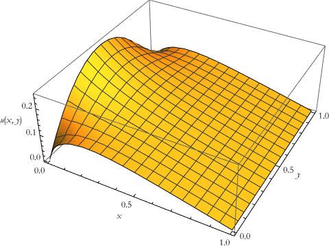
We can get a solution we can plot. Take the first 5 terms of the series.
![]()
![]()
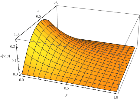
The plot of this is then given here.
![]()
DEigensystem and NDEigensystem
There is a system for finding the eigenvalues and eigenfunctions of an operator on some region. For the problem above we can write the operator.
![]()
![]()
We then need to specify our Dirichlet boundary conditions.
![]()
We then apply the command DEigensystem to establish the smallest ten eigenvalues, denoted eval1, and the eigenfunctions, denoted efun1, on a rectangle.
![]()
Here is the list of eigenvalues.
![]()
| 1 | |
| 2 | |
| 3 | |
| 4 | |
| 5 | |
| 6 | |
| 7 | |
| 8 | |
| 9 | |
| 10 |
Here we have a table of the eigenfunctions.
![]()
| 1 | 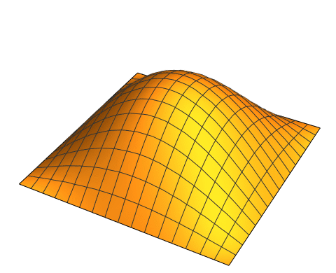 |
| 2 | 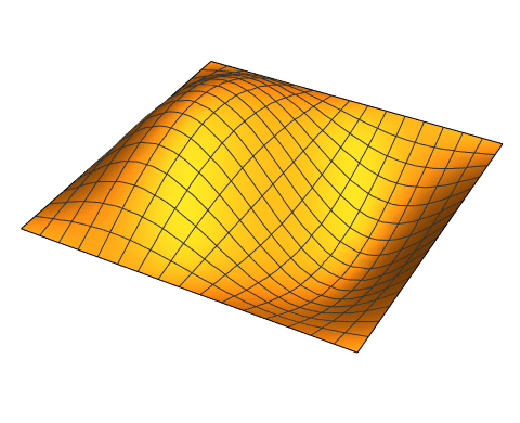 |
| 3 | 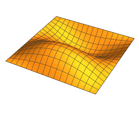 |
| 4 |  |
| 5 | 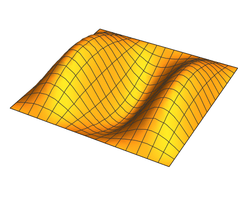 |
| 6 | 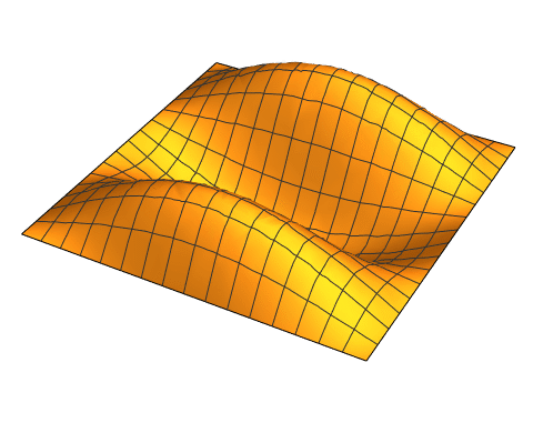 |
| 7 |  |
| 8 |  |
| 9 |  |
| 10 |  |
We can also perform a numerical approximation.
![]()
Here is the list of eigenvalues.
![]()
| 1 | -19.7392 | -19.7392 |
| 2 | -49.348 | -49.3486 |
| 3 | -49.348 | -49.3486 |
| 4 | -78.9568 | -78.9579 |
| 5 | -98.696 | -98.7021 |
| 6 | -98.696 | -98.7021 |
| 7 | -128.305 | -128.311 |
| 8 | -128.305 | -128.311 |
| 9 | -167.783 | -167.817 |
| 10 | -167.783 | -167.817 |
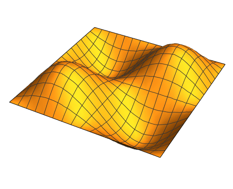
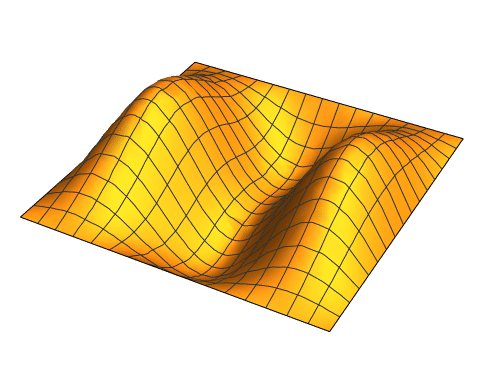
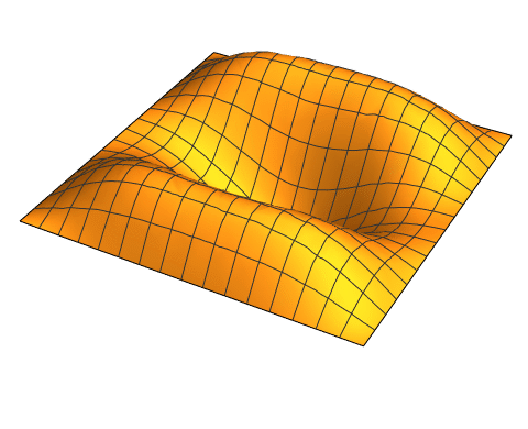
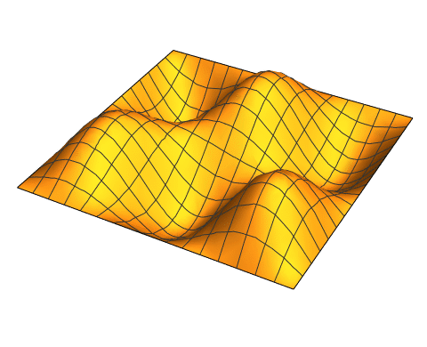
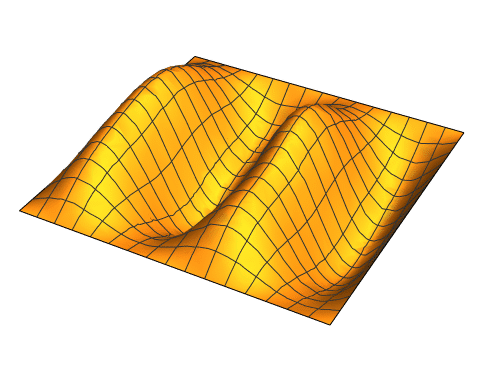
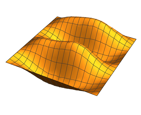
Here we have a table of the eigenfunctions.

| 1 |  |
 |
| 2 |  |
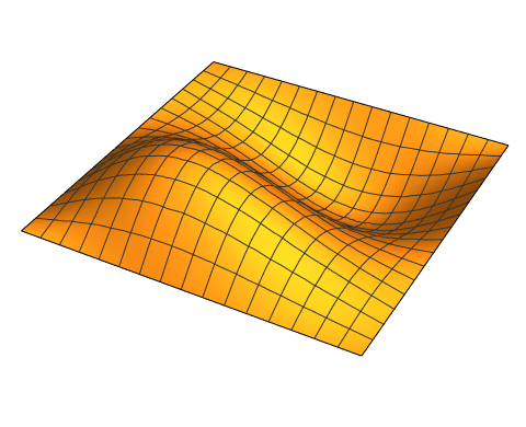 |
| 3 |  |
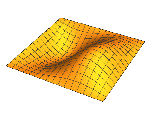 |
| 4 | 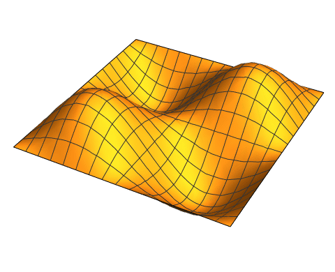 |
 |
| 5 |  |
 |
| 6 |  |
 |
| 7 | 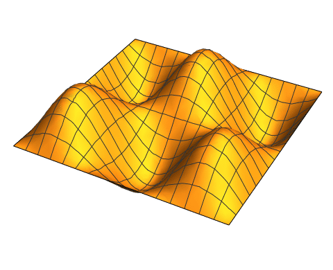 |
 |
| 8 | 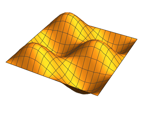 |
 |
| 9 | 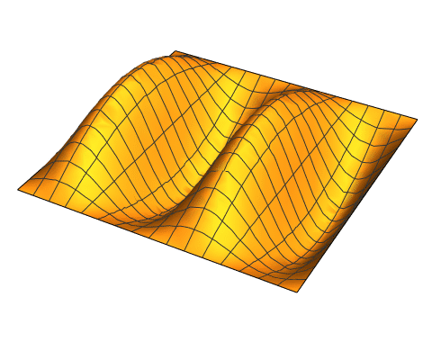 |
 |
| 10 | 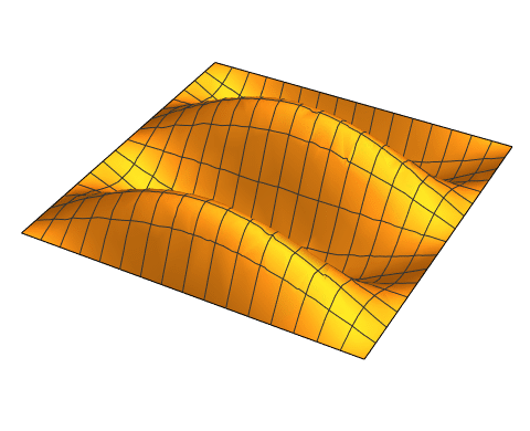 |
 |
Neumann Problems
Here we examine the solution of the Laplace equation with both Dirichlet and Neumann conditions. Here we specify the Neumann conditions.
![]()
![]()
Then we build the solution.
![]()
![]()
We can get a solution we can plot. Take the first 5 terms of the series.
![]()
![]()
The plot of this is then given here.
![]()
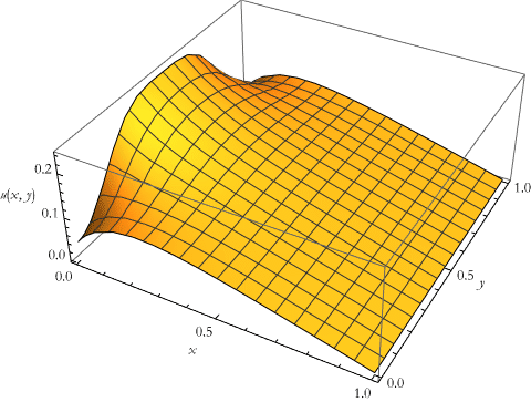
Here is the numerical solution.
![]()
![]()
![]()
![]()
So, we then have to write this.
![]()
![]()
![]()
![]()
![]()
Specific Regions
We are not restricted to rectilinear regions. Any region that you can specify using the Region command can be used. There are many preset regions. For example, we produce the solution of a potential on a disk. We write the Laplace equation in polar coordinates.
![]()
![]()
Now we want to solve the Dirichlet problem for the disk. We write the boundary conditions.
![]()
Now we write the solution.
![]()
![]()
![]()
![]()
We extract the first five terms of the series.
![]()
![]()
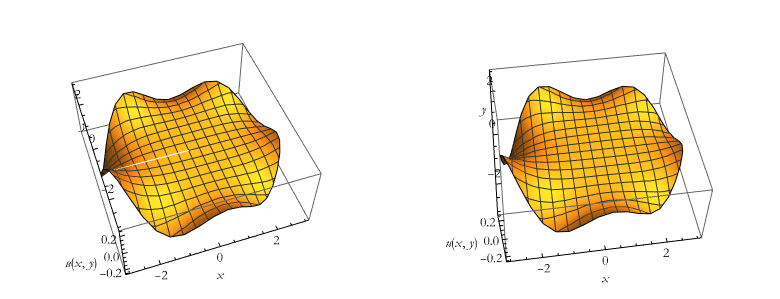
Here is a plot of this over the disk.
![]()
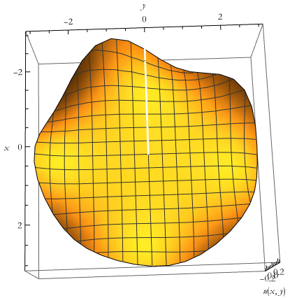
![]()
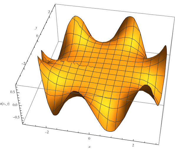
Note that there is an exclusion in these plots, we can remove them.
![]()
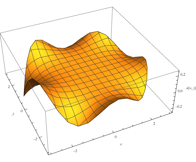
Note the distortion where the two parts of the disk are “glued” together.
![]()
Unbounded Regions
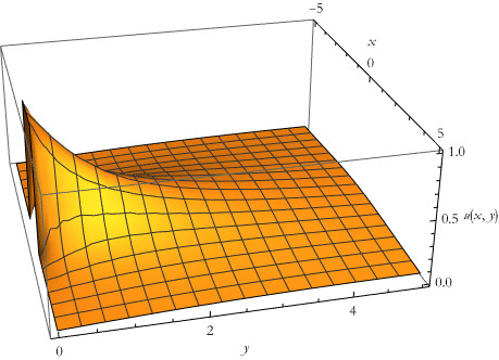
We are not restricted to finite regions, either. Here we consider the first equation (9.1) on an upper half plane characterized by the Heaviside step function θ for y>0. This being the case, our boundary value will be,
![]()
(9.4)
We write this.
![]()
So our solution will be given as.
![]()
![]()
The plot of this will be.
![]()
The Poisson Equation
The Poisson equation is similar to the Laplace equation, except that it is not homogeneous,
![]()
(9.5)
where f is defined for the problems at hand. For example, if we are studying the Poisson equation for gravitation f would be replaced by the mass density of the problem. Here we set up such an equation.
![]()
Here are some boundary conditions on a rectangle.
![]()
![]()
![]()
![]()
Now we build the solution.
![]()
![]()
We extract the first five terms.
![]()

The plot of this will be.
![]()
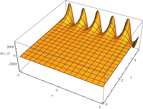
It looks pretty flat until we look at the vertical scale. Let’s look at the plot for less than 5 in y.
![]()
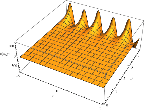
Now let’s try it for a maximum of y=4.
![]()
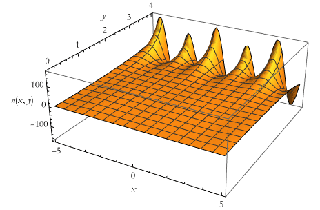
How about max y=2?
![]()
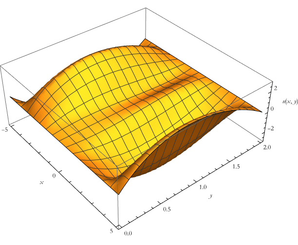
It is an interesting potential function.
Sources and the Inhomogeneous BC
What happens when we have a source of potential on a boundary? Let’s put in a quadratic source term in the boundary conditions,
![]()
(9.6)
and at the other side
![]()
(9.7)
Here we write the boundary conditions.
![]()
![]()
We then construct the solution.
![]()
![]()
We extract the first five terms.
![]()
![]()
The plot of this will be.
![]()
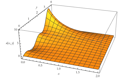
Three Dimensions
Here we modify the Laplace equation into three dimensions,
![]()
(9.8)
If we decide to solve this over a rectangular parallelepiped we write our equation and boundary conditions.
![]()
![]()
![]()
![]()
We now construct the solution.
![]()
| |
|
We can plot this solution using a ContourPlot3D. Note that we here are considering the first ten terms of the series.
![]()
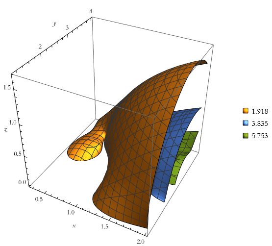
Other Coordinates
We have already seen how to use polar coordinates. Here we examine the Laplace equation for a potential between two spheres of radius ![]() and
and ![]() . The potentials will then be between the values
. The potentials will then be between the values ![]() and
and ![]() .
.
![]()
![]()
We write our Dirichlet condition.
![]()
We then write the solution.
![]()
| |
|