Fourier Analysis and Laplace Transforms

George E. Hrabovsky

MAST

Introduction

In the last lesson we saw how several PDEs in DSolve resulted in an answer involving Fourier series. In this lesson we examine how Mathematica handles Fourier series and Fourier transforms. We will then discuss Laplace transforms.

Fourier Series

How do we generate a Fourier series in Mathematica? We use the FourierSeries command.

The nth-order Fourier series has the form,

(8.1)

where the coefficients are given as,

(8.2)

In general, if we have a differential operator L such that for the functions u and v L(u+v)=L(u)+L(v) and for the constant or parameter c L(c u)=c L(u) then we say that the operator is linear. Any operator that is not linear is called nonlinear. It turns out that we can write any linear differential equation using a linear operator

So what does the output look like? Here is the second-order Fourier series for t.

We can see the role of the Parameters by specifying their values as {a,b}.

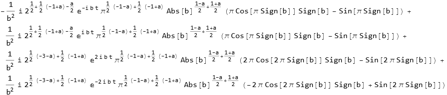
The default values are {1,1}. Here is what happens when we apply the condition that the parameters are {1,2 π}.

Here is a plot of this.

Here we see five zeros. How do we know these are zeros and not just poles? Zeros go from -π to π in a counterclockwise manner. Poles go clockwise.

We can also find the Fourier sine series.

And we can find the cosine series.

We can even find the Fourier coefficients. Here we have a table of the first five coefficients.

1
2
3
4
5

Here are the first five Fourier sine coefficients.

1
2
3
4
5

Here are the first five Fourier cosine coefficients.

1
2	0
3
4	0
5

As an exercise work through the documentation on FourierSeries, FourierCoefficient, FourierSinSeries, FourierSinCoefficient, FourierCosSeries, FourierCosCoefficient and work through some examples.

Fourier Transforms

We can also perform Fourier transforms.

Compare this result with the Fourier series above .

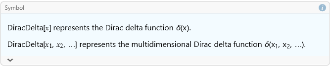
Note that this result is the frequency derivative of the Dirac delta.

We can always transform an elementary function.

Here the Sign function is defined.

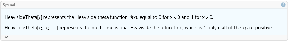
We can also transform special functions.

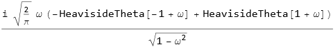
Periodic functions are what you would expect. Here we transform a common result.

We can also use the Fourier sine transform.

And the Fourier cosine transform.

We can also perform an inverse Fourier transform.

As an exercise read through the documentation on FourierTransform, FourierSinTransform, FourierCosTransform, InverseFourierTransform, InverseFourierSinTransform, and InverseFourierCosTransform and work through several examples.

Discrete Fourier Analysis and Spectral Methods

So far, all of this has been about Fourier analysis of defined expressions. What about data? In such a case we use the command Fourier. Let’s say that we have some noisy data.

We can see a plot of this.

So, we can apply a discrete Fourier transform on the data.

Now we can plot that .

Too zoomed in for us to see anything, what happens when we expand the view.

We see a very strong spike at a little over a hundred. We see a corresponding, symmetric, spike at a little less than a hundred from the far end.

We can also find the power spectrum of the data. What is that? It is the magnitude of the Fourier transform.

As an exercise read through the documentation for the commands Fourier and Periodogram and work some examples.

As an exercise read through the section Discrete Fourier Transforms of the technical note Numerical Operations on Data, look up the documentation on any new functions in that section, and work some examples.

Laplace Transforms

Fourier transforms take an input function, applies a function called a kernel, and the output function is of a different variable. Such a transform is termed an integral transform, since the application of the kernel to the input function is integrated with respect to the input variable. Another kind of integral transform that is very useful is the Laplace transform. Why use a Laplace transform? Laplace transforms allow you to incorporate initial conditions. It can transform a differential equation into an algebraic equation, you can then solve that algebraic equation, and then apply an inverse Laplace transform to convert the algebraic solution into the solution of the differential equation. [Note about the initial condition as opposed to Fourier transforms].

Here we write an inhomogeneous ODE.

We apply a Laplace transform to convert t to s.

As you can see we have opportunity to define the initial conditions. Let’s assume that the initial conditions are both 0.

We now solve this weird equation for the Laplace transform.

We now apply an inverse Laplace transform to this.

Compare this to the direct solution.

As an exercise read through the documentation for LaplaceTransform and InverseLaplaceTransform and work some examples.

As an exercise read through the tutorial Integral Transforms and Related Operations and work some examples.

Note that we will discuss the Z transform when we get to solving difference equations in a later lesson.