Partial Differential Equations

George E. Hrabovsky

MAST

Introduction

We have spent half the course up to now talking about ODEs. We now shift our attention to partial differential equations (PDEs). Mathematica has many tools for handling PDEs. The documentation is quite extensive on this topic. To be clear, a PDE is one having partial derivatives of one or more functions of more than one variable.

We will adopt the convention of writing derivatives as subscripts of the function label in terms of the independent variable the derivative it is with respect to.

(7.1)

Any function f that satisfies the conditions of a given PDE is said to be a solution of that PDE.

We will also adopt a convention of writing a general function of each of its arguments as an upper case letter, such as F. So a generic PDE can be written F(...)=G(...).

We can think of any differential equation as the application of a differential operator L to the function of our variables (or functions of our variables). Thus we can write a PDE as L(f)=F(...)=G(...).

Classification

The subject matter of PDEs and their solution is truly vast. One way to get a handle on such a huge subject is to classify the equations, allowing us to narrow our methods and theory.

The first classification is the highest-order partial derivative in the PDE, that defines the order of the PDE. For each order of a time derivative in a PDE we need to define an initial condition.

The second classification is in terms of the number of independent variables. In two independent variables, say x and t, we can write the most general first-order PDE,

(7.2)

In a similar way we write the most general second-order PDE in two variables,

(7.3)

Another criterion for classification is the nature of the coefficients, if they are constants then we call the PDE a constant coefficients PDE. Otherwise we call it a variable coefficients PDE.

If an equation is a linear combination of a function u and its derivatives then we call it a linear PDE. This works for ODEs too. Any equation that is not linear is called nonlinear.

In general, if we have a differential operator L such that for the functions u and v L(u+v)=L(u)+L(v) and for the constant or parameter c L(c u)=c L(u) then we say that the operator is linear. Any operator that is not linear is called nonlinear. It turns out that we can write any linear differential equation using a linear operator

Another criterion for classifying PDEs that we will consider here is the nature of G in the statement L(f)=F(...)=G(...). If G is identically 0 then the equation is homogeneous. Any PDE that has it defined by a linear operator that is homogenous is a linear PDE. If an equation is not homogeneous it is inhomogeneous. If a differential equation is linear and you have two solutions, then the sum of those solutions is another solution. This is called the superposition principle. It applies to ODEs and PDEs.

Boundary Conditions

It is rare to find applications of PDEs that do not involve some kind of region where the solution needs to be found. If we symbolize the region with the Greek letter omega, Ω, we may then write its boundary as ∂ Ω. A wave propagating along a string is confined to the region of the string, for example. The endpoints of that string are the boundaries of the region. We will consider several types of boundary conditions.

The first kind of boundary condition we will consider is one where a specific value exists at the boundary. This is called a Dirichlet condition, named for work done by the German mathematician and physicist Peter Gustav Lejeune Dirichlet (1805-1859) published in 1828. Such Dirichlet conditions are usually in the form of some equation. There is also a Mathematica command that you can use with DSolve to establish Dirichlet conditions, it is (reasonably enough) called DirichletCondition[boundary equation,predicate], where the boundary equation is active when the predicate is met. We will see examples of this kind of boundary condition later, and we will examine the Mathematica command in later lessons. The act of finding a solution of this type is called a Dirichlet problem.

The second kind of boundary condition is one where there is a flux that is normal to the boundary defined as a partial derivative. What do we mean by normal? If we write as the unit normal vector on the boundary pointing outward from the region, then we define a normal derivative in terms of the unit normal vector and the directional derivative,

(7.4)

If

(7.5)

then (7.5) holds at the boundary then we have what we call a Neumann condition, named for the German mathematician Carl Neumann (1832-1925). In Mathematica there is a command called NeumannValue[value,predicate] that adopts the value whenever the predicate is met. This command is added to the existing PDE in DSolve. We will see examples of this later. The act of finding a solution of this type is called a Neumann problem.

The third kind of boundary condition arises when both the value of function u and its normal derivative are specified, then we call that a Cauchy boundary condition, and we call its solution a Cauchy problem. It is named for the French mathematician, physicist, and engineer  Augustin-Louis Cauchy (1789-1857).

The fourth kind of boundary occurs where both a linear combination of the values of function u and its normal derivative are specified,

(7.6)

This is called a Robin condition, named for the French mathematician Victor Gustave Robin (1855-1897). It is interesting that we can use the NeumannValue command for Robin type boundary conditions, too.

The situation can exist where different boundaries of the same system have different, and disjoint, boundary conditions. Such a situation is called a mixed boundary condition.

It is also important to realize that these boundary conditions apply to ODEs and not just PDEs.

Examples

The simplest PDE is, given u(x,y)

(7.7)

Solutions of this equation are of the form

(7.8)

so whatever function we are applying to y is constant across x.

We can write a first-order equation with constant coefficients,

(7.9)

By the method of characteristics, the characteristic curves for this equation satisfy the ODE

(7.10)

This is a simple ODE to solve,

(7.11)

By the nature of characteristic curves we know that u(x,y)=f(c).  Solving (7.11) for c we get,

(7.12)

so the solution of (7.9) is

(7.13)

We can also write a first-order equation with variable coefficients.

(7.14)

If we again apply the method of characteristics, we get the ODE

(7.15)

The solution of this ODE is

(7.16)

and these are the characteristics. Solving for c gives us

(7.17)

The solution to (7.14) is then,

(7.18)

DSolve

Of course, we can use DSolve with PDEs in a manner similar to ODEs. Here we see the solution to our simplest PDE.

This is what we expected to see, the solution is some arbitrary function of y. What happens if we integrate this again?

Now we have the solution in terms of two arbitrary functions of y. We can examine some boundary value problems for this equation, too. Let’s say that whenever x=0 that u(x,y)=cos y/2.

Note that the boundary function replaces our arbitrary function.

Let’s try to solve the equation in (7.9). This is a slight modification of the example from the documentation.

We can use the same sort of solution for (7.14).

We can specify this arbitrary function using the rule-delayed command :→.

As an exercise read through the section on First-Order PDEs in the Scope section of the write up on DSolve.

As an exercise read through the sections Overview of PDEs and First-Order PDEs in the section PDEs in the tutorial Symbolic Differential Equation Solving.

As an exercise read through the Introduction to the tutorial Symbolic Solutions of PDEs.

DSolveValue

This is a command that does much the same thing as DSolve, but it does not return a rewrite rule like DSolve, it just returns a value. For example.

This negates the step of writing exp1 above.

As an exercise read through the write up for DSolveValue.

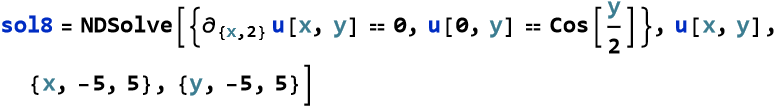
NDSolve

We can also apply the NDSolve command we used for ODEs. Again, the result is an interpolating function. For example, we can numerically solve our simplest PDE.

Note the two warning messages. Convection-dominated PDEs are characterized by highly irregular solutions. What does that mean? It means there might be jumps, kinks, or other kinds of discontinuity. Let’s plot this and see what is happening.

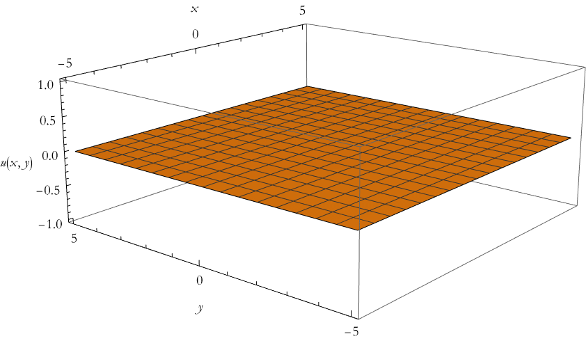
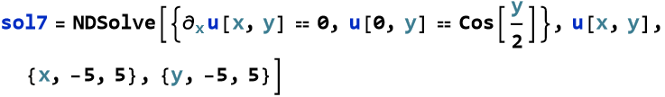
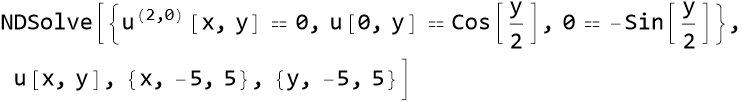
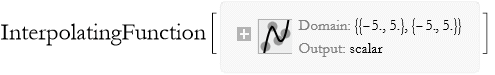
This is weird, there seems no value. Let’s look at the second message. It is suggesting some kind of boundary condition. Let’s say that we have the same condition we had above, whenever x=0 that u(x,y)=cos y/2.

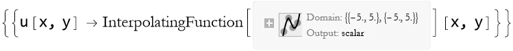
So the introduction of an initial condition seems to have solved the problem. Here is the new solution plot.

What was the issue with the convection-dominated PDE message? The answer is based on an arbitrary function that is not defined.  Without an initial condition the solution surface is flat.

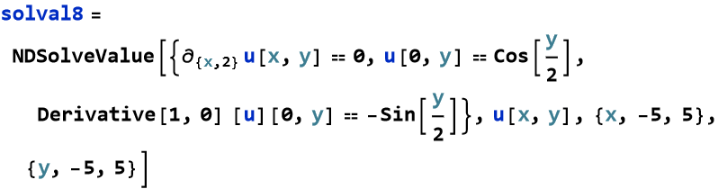
We need to do the same thing a second time for our second PDE from above.

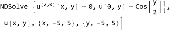
What do we use as a second constraint?

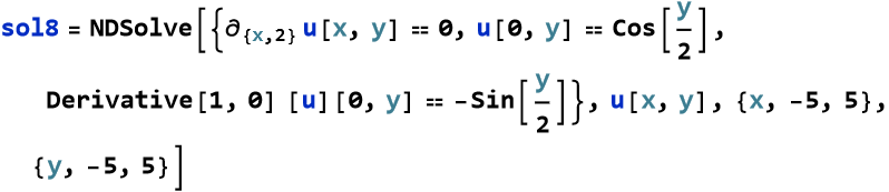
Why not just write the derivative ? Let’s see what happens.

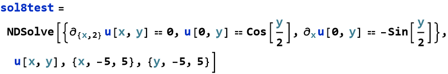
So, if you have an initial condition that does not seem to be working, try to change the way it is written. As an exercise look up the Derivative command and work through some examples.

For the solution that returned a result, here is the plot.

NDSolveValue

NDSolveValue has the same relation to NDSolve as DSolveValue has to DSolve. It does not return a rewrite rule, it just returns an interpolating function.

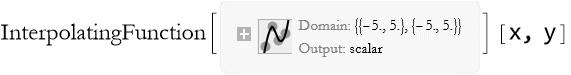
Note the difference in the plot.

Another Level of Classification

Many PDEs of interest are of higher than first-order. Let’s assume a function u(x,y) and a generic homogeneous second-order PDE is

(7.19)

We choose a trial function f, that is twice differentiable, of the form

(7.20)

We then find the relevant second-order partial derivatives for our PDE,

(7.21)

Substituting this into (7.19) gives us

(7.22)

There are three cases we can consider, f''=0, , or both.

If we look at the case f''=0, then we have the solution . This requires two arbitrary constants instead of two arbitrary functions and is thus not the most general solution. We may thus disregard this as a solution.

This leads us to consider the case , where we can choose a linear combination of the variables x and y and get a solution for any twice differentiable function f. This is a quadratic equation leading to the solutions

(7.23)

The sign of the discriminant is extremely important in determining the number and type of solutions to the quadratic. There are three broad cases

(7.24)

In the case , there are two distinct real solutions. PDEs of this type reduce to the form and are called hyperbolic.

In the case , there is a single degenerate root. PDEs of this type reduce to the form and are called parabolic.

In the case , there are two distinct complex roots. PDEs of this type are called elliptic.

Almost all of the PDEs used in theoretical physics fall into one of these categories. We shall cover each of these three kinds of equations in their own lessons later.

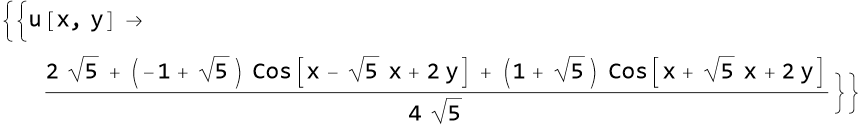
An Example of a Hyperbolic PDE

Here is an example of a second-order hyperbolic PDE in DSolve.

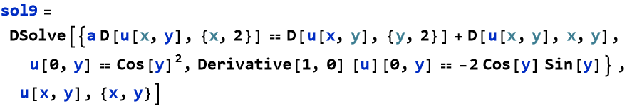
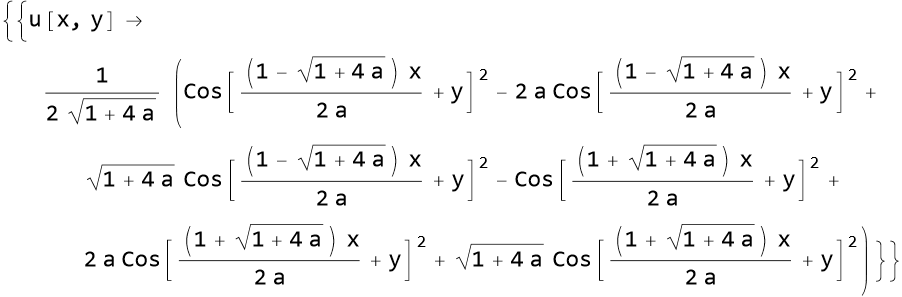
The solution surface can be  plotted, here we assume a=1.

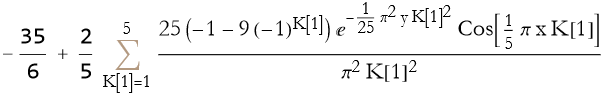
An Example of a Parabolic PDE

Here we have a parabolic type PDE.

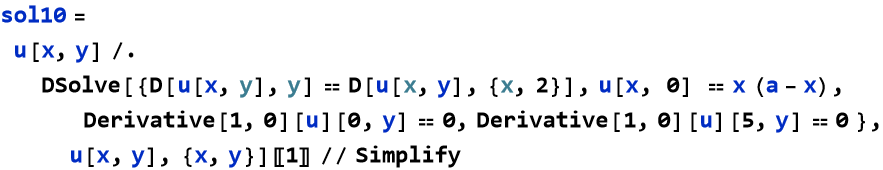
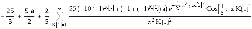
This takes a while. The answer is in the form of a Fourier cosine series. We can get the first five terms.

We can plot this.

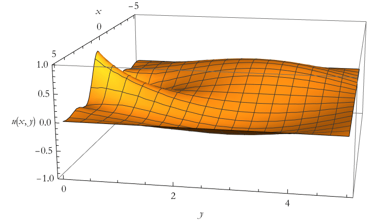
An Example of an Elliptic PDE

Here we have an example of an elliptic PDE. Our PDE will be a Helmholtz-type equation on a rectangle. Here we introduce the Laplacian command and the UnitTriangle.

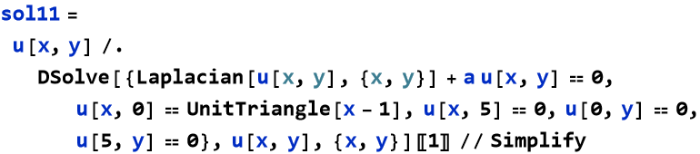
We again have an answer in the form of a Fourier series. We will take the first few terms and assume a=1.

Here is the plot of this function.

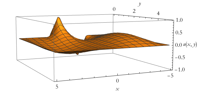
What happens if we get more terms in the series?

Time-Dependent Problems

Up to now we have dealt primary with PDEs having only spatial derivatives. Many situations involve processes that evolve in time, what we now call a dynamical system. This allows us to consider problems of the form

(7.25)

Such an equation is called a conservation law. Here is a good example of a time-dependent PDE. We can write the wave equation for some velocity v, and for some function u(x,t),

(7.26)

So we have second derivatives instead of first derivatives. Is this still a conservation law? If we multiply by we get,

(7.27)

We can factor this,

(7.28)

Here we have two operators acting on the function. If we impose the condition that,

(7.29)

this effectively destroys the second operator in (7.28), and (7.29) satisfies the wave equation in (7.26). This is a conservation law. Can we find a general solution to (7.29)?

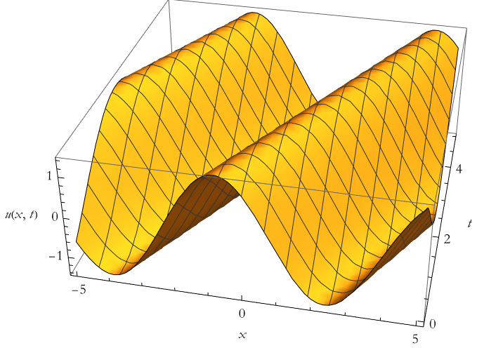
This is a fairly well known result. This is very familiar as we have a solution of a constant function and is another example of the method of characteristics. We can impose a function form here and we assume the wave velocity to be 1.

Here we can plot the time evolution of this wave,.

What's Going On Under the Hood?

The command NDSolve hides a lot of complications. In order to approximate the integration of a PDE we must first establish a grid, or mesh, covering the region we are concerned with. The vertices of this mesh (and it need not be rectilinear) form the cells of a matrix. This discretization of a spatial region into a matrix turns the problem of solving a PDE into a problem of solving a really large, and often complicated, matrix equation. The elements of this matrix equation are often created by some scheme such as finite differencing, like what we saw in Lesson 1.

Broadly speaking there are two kinds of  meshes. The first is a fixed mesh. Here the distance across one cell is the same throughout the solution of the PDE. The second is an adaptive mesh, and we will discuss that in a later lesson, when we talk about the finite element method. For now we can say that an adaptive mesh changes, or adapts, to the current situation.

It is possible to have a finer mesh for areas of particular interest to your study. That is called a nested grid. The danger of a nested grid is that you can propagate artifacts of instability outside of the finer grid.

The ability to make meshes is important to Mathematica, and we will discuss this in greater detail when we get to the Finite-Element method in a later lesson.