Matrix and Vector Operations

George E. Hrabovsky

MAST

Introduction

We have already seen how to use matrices in terms of data analysis. Here we will review some of the basics in terms of how to use Mathematica to solve problems involving both matrices and vectors.

Constructing Matrices

How do we enter a matrix into Mathematica? The simplest way is to go to the Insert menu above. Choose Table/Matrix. Then choose New. Click Matrix. Then specify the number of rows and columns. I chose 2 each. Then click on OK. This is what you get.

You can enter what you like into the spaces.

The limitation of this method becomes apparent in two cases. The first is if the matrix is large. The second is if the matrix has definite values based on some method or process.

For these situations we use the Table[] command. For example, if we have a 3×3 matrix whose elements are given by a formula, then we might write what follows.

We can see this in matrix form.

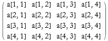
We can also use the Array command.

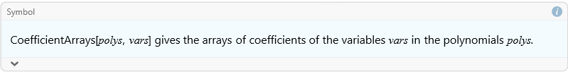
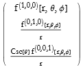
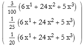
We can construct an array of the coefficients of a list of polynomials using the CoefficientArrays command.

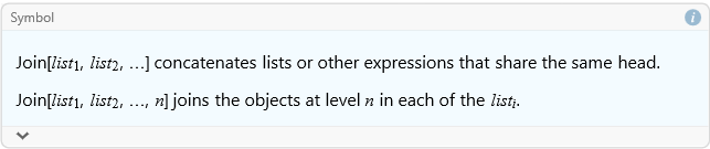
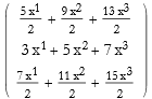
We can combine two matrices by using the Join command.

Elements and Shapes of Matrices

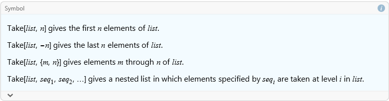
We can use all of the list commands to pull out the elements of a matrix. Here we take the third row of our first matrix.

Here is the second column.

We can also get a submatrix using the Take command.

We can also take pieces away from a matrix to make a new matrix by using the Drop command.

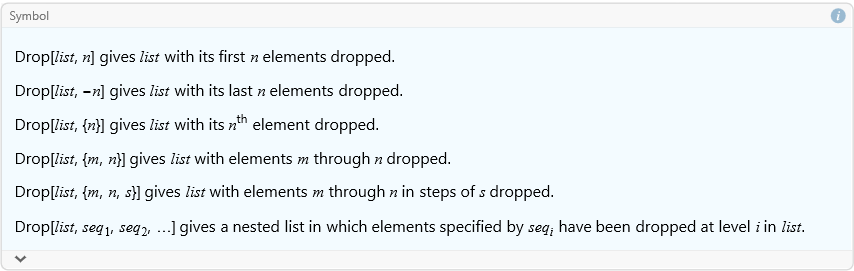
Here we remove the first row from exp1.

Here we remove the first column.

If we want only particular parts of a matrix we use the Extract command.

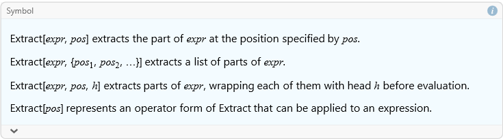
Here we extract the first row from exp1.

Here we remove the first column.

Given a full array, one whose rows and columns form a rectangular array, we can get a list of the dimensions of the array using the Dimensions command.

An array that is not full is sometimes termed ragged.

In this last case the first row determines the size of the array, the other rows do not have the same number of elements, so we call this ragged.

We can extract the diagonal of a matrix using the Diagonal command.

We can transpose a matrix.

Transpose can also be accomplished by typing [ESC]tr[ESC]

As an exercise read through the documentation on Transpose and work several examples.

What about the Hermitian (or Conjugate) Transpose? We can use [ESC]ct[ESC], or the command ConjugateTranspose[].

This is not a good test as there were no complex numbers.

As an exercise read through the documentation on ConjugateTranspose and work several examples.

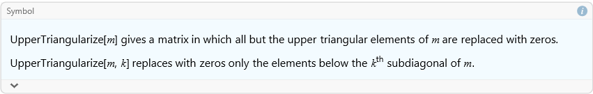
If we want to keep all of the upper triangular elements as they are, but all other elements become zeros we use the command UpperTriangularize.

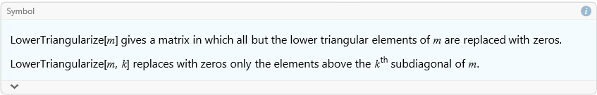
We can do a similar thing with the LowerTriangularize command.

It is also possible to change an element of a matrix using the ReplacePart command.

For example, we can change exp14 to have a 4 in the {1,3} position.

Vectors

From the perspective of lists and matrices, a vector can be represented as a one-dimensional matrix, either a column or a row. In fact, the default representation of a vector is written as a row, but it is treated as a column vector. Any method that allows you to make a matrix can, therefore, be used to construct a vector.

This seems to be a row matrix, but if we apply MatrixForm we see that it is a column matrix.

A row matrix is constructed this way.

We can also create a vector field from a scalar field by taking its gradient.

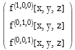
We can also use other coordinate systems.

We can do the same thing with the keyboard combination  [ESC]del[ESC] followed by [CTRL]_ to list the variables.

Matrix-Vector Multiplication

In lesson two we examined how to multiply a vector by a matrix. We can use the same notation for matrices in general. For example

We can see that the order of multiplication is important.

Vector Operations

Let’s say  that we define another vector.

We can add vectors.

Scalar multiplication is accomplished in a completely intuitive way.

The scalar product is accomplished using the . symbol.

You can also use the Dot command.

The vector product is accomplished using the combination [ESC]cross[ESC].

You can also use the Cross command.

We can find the norm of a vector using the Norm command.

We can also evaluate the norm of a numerical matrix.

If we have a symbolic matrix

We can write its norm.

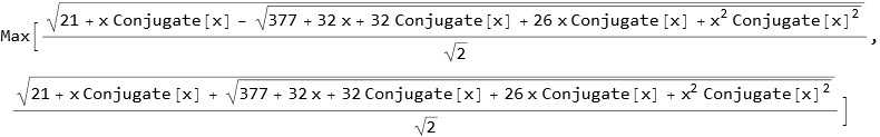
We can restrict this to the reals to eliminate the conjugation.

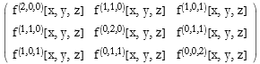
We can get the Jacobian matrix by taking the gradient of a vector field, in this case it is the Hessian because it is the gradient of a gradient.

We can also make this specific.

We can find the divergence of a vector field by using the Div command. If our generic vector field is composed of three functions of the coordinates we write the field.

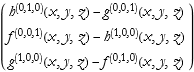
The divergence of this field in Cartesian coordinates is then calculated.

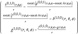
We can also produce the divergence in spherical coordinates.

We can find the Curl of a vector field via the Curl command.

Here we have spherical coordinates.

Say we have another vector.

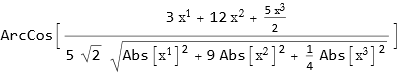
We can find the angle between vectors by using the VectorAngle command.

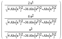
We can use Normalize[] to find the unit vector in the direction of vec1.

How do we project vec1 onto vec2?

How do we find an orthonormal set of vectors for these two vectors?

This takes a little bit of time.

As an exercise look up the documentation on Normalize,  Projection, and Orthogonalize and work several examples of each.

Matrix Operations

In lesson 2 we introduced both matrix multiplication and the Inverse command for inverting a matrix. Here we can see a plot of these commands.

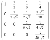
As another example, we make a 4th-order square Hilbert matrix.

As an exercise read through the documentation on Inverse and MatrixPlot (and also ArrayPlot), and work several examples.

In lesson 2 we saw how to calculate a determinant. Here is a program from the Wolfram documentation on how to calculate the cofactor of a square matrix.

We use this to find the cofactor of exp11 removing the 3rd row and second column.

As an exercise read through the documentation of Det and work several examples.

We can also find the minors of a matrix.

We can also use this on symbolic matrices.

Here we compare it to the original matrix.

As an exercise read the documentation for Minors and work several examples.

We can use this program from the documentation to find the adjoint of a matrix.

Here we find the adjoint of the two examples.

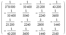
In the new version of Mathematica (version 13) there is a new command, Adjugate.

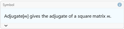
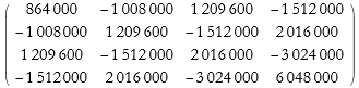
Adjugate is another name for the classical adjoint. We can compare the results with the ones from above.

We can find the trace of a matrix.

As an exercise read the documentation for Tr, note particularly the program for calculating the inner product of a cone of positive definite matrices. Work several examples of your own.

We can calculate powers of matrices.

As an exercise read the documentation for MatrixPower, note particularly the application for composing a set of infinitesimal rotations to determine a finite rotation matrix. Work several examples of your own.

We can also calculate matrix exponentials.

As an exercise read the documentation for MatrixExp, note particularly the application for determining the basis for the general solution of a system of ODEs. Work several examples of your own.

Linear Systems

A common problem is how to solve a system of linear equations. We say that you could use the LinearSolve command to solve a matrix equation for a solution vector. There are different methods that can be used.

Say we use our matrix in exp31.

We construct a matrix equation.

We can use Solve on this system .

Let’s see what happens when we use LinearSolve.

As an exercise read through the documentation on LinearSolve, note (and try out) the neat examples of 100,000 equations (taking a little more than a tenth of a second) and then 1,000,000 equations (taking about 1.4 seconds).

As another exercise read through the section Solving Linear Systems in the tutorial Linear Algebra. Work through some examples.

Eigenvalues and Eigenvectors

We can find the eigenvalues of a matrix.

As an exercise read through the write-up of Eigenvalue and work up some examples.

We can also find the eigenvectors.

We can use this to diagonalize the matrix.

As an exercise work through the documentation for Eigenvectors and work several examples.

We can find the characteristic polynomial for a matrix by using the CharacteristicPolynomial.

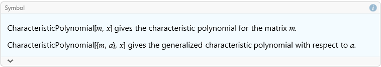
Singular Values and Matrix Norms

Want to find a list of singular values for a matrix?

As an exercise read through the write up for SingularValueList and work some examples.

Related to this is the matrix norm. The theory of matrix norms is extensive, and beyond the scope of this lesson. Assuming that you have a need to find the n-norm of a matrix, we use the Norm command. This is the same Norm command we used for vectors.

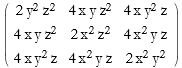
We can also find the Frobenius norm, this is the square root of the trace of the matrix A formed by A A.

As an exercise read through the write up for Norm and work some examples.

Other Decompositions

In lesson 2 we discussed several schemes for decomposing matrices. We will now consider additional methods. The Cholesky decomposition of a matrix A returns an upper triangular matrix U such that UU=A.

The Jordan decomposition takes a square matrix A and returns a similarity matrix S and the Jordan canonical form J such that .

We can place this into matrix form.

The first matrix is S the second is J.

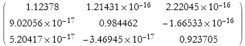
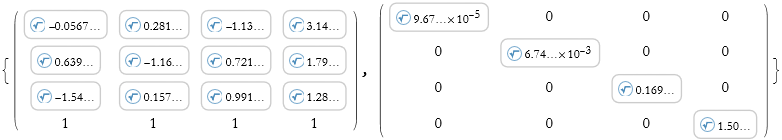
The Schur decomposition takes the matrix A and returns the orthonormal  matrix O and the upper triangular matrix U, such that A=O U O.

The Hessenberg decomposition takes the matrix A and returns the unitary matrix P and the upper Hessenberg matrix H such that A=P H P.

Abstract Vectors and Matrices

In lesson 3 we introduced the abstract Vectors command. There is a similar command for Matrices.

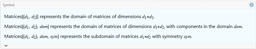
We can define a class of matrices symbolically.

We can check to see if a matrix is a member of a set of matrices.

We can also use this to simplify conditions.