Special Functions
George E. Hrabovsky
MAST
Introduction
We have seen examples of solutions of ODEs resulting in the application of special functions. In this lesson we will explore some of their basic ideas. We will also discuss how they are implemented in Mathematica.
Series Solutions of ODEs
One frequently used method of solving ODEs that has been missing from Mathematica (though it was always possible to construct a solution that produced these results) is the method of power series expansions. Constructing the solution was not straightforward and had to be done in detail for each problem anew. Starting with version 12.1 a new function was added that let’s you do this using the AsymptoticDSolveValue. Here is our harmonic oscillator equation as an IVP centered at the origin.
![]()
![]()
We can plot this solution.
![]()
It works well up to 2 π, but beyond that it begins to get errors. We can see a set of successive approximations by a combination of the Accumulate and List mapping commands.
![]()
The nice thing about this function is that it detects the nature of the point (ordinary and regular or irregular singular points) and applied the correct method (Taylor series or Frobenius). The method can be used with a small parameter to get a perturbation series, and if you set a limit of infinity it will give you an asymptotic expansion.
How do we tell if a point is ordinary or singular? Let’s say that we Taylor expand a function of x around the point ![]() ,
,
![]()
(5.1)
If the function is infinite differentiable at ![]() and it also satisfies (5.1), then function is called an analytic function, or sometimes a regular function. Now, say that we have an ODE of the form
and it also satisfies (5.1), then function is called an analytic function, or sometimes a regular function. Now, say that we have an ODE of the form
![]()
(5.2)
If both ![]() and
and ![]() are analytic at some point
are analytic at some point ![]() , then the point
, then the point ![]() is said to be ordinary. A point that is not ordinary is called singular. If a point is singular and the products
is said to be ordinary. A point that is not ordinary is called singular. If a point is singular and the products ![]() and
and ![]() are both analytic at
are both analytic at ![]() , then the point
, then the point ![]() is called a regular singular point for the second-order equation. Otherwise it is called an irregular singular point. Can we get Mathematica to help us find these points?
is called a regular singular point for the second-order equation. Otherwise it is called an irregular singular point. Can we get Mathematica to help us find these points?
We can convert a second-order equation into the form of (5.2) and test to see if the functions ![]() and
and ![]() are analytic. Take the equation in sol1, we can write it
are analytic. Take the equation in sol1, we can write it
![]()
(5.3)
where ![]() and
and ![]() . We can use the command FunctionAnalytic to test these.
. We can use the command FunctionAnalytic to test these.
![]()
![]()
![]()
![]()
Thus, any point chosen is an ordinary point. Let’s see what happens if we choose our regular point to be 3 π.
![]()
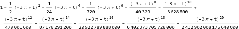
The plot for this solution now looks like this.
![]()
So it is doing pretty well near the regular point.
What about the equation,
![]()
(5.4)
does it have ordinary or singular points. We again rewrite the equation,
![]()
(5.5)
where ![]() and
and ![]() . We can use the command FunctionAnalytic to test these.
. We can use the command FunctionAnalytic to test these.
![]()
![]()
![]()
![]()
So we have at least one singular point. How do we tell where this point is? We can try to use FunctionSingularities[].
![]()
![]()
So, there is a singular point at ![]() . Is it regular or irregular? If we multiply
. Is it regular or irregular? If we multiply ![]() by
by ![]() , we still get 0, so that is analytical. What about
, we still get 0, so that is analytical. What about ![]() ? If we multiply that we get
? If we multiply that we get ![]() .
.
![]()
![]()
So the singular point is regular.
As an exercise read through the AsymptoticDSolveValue command write up, and come up with some examples.
Gamma and Beta Functions
The gamma function has an extensive treatment in Mathematica. The Gamma function is an integral-defined function.
![]()
(5.6)
Here we plot the gamma function over a real domain.
![]()
Here we plot it over a complex domain.
![]()
From pl1 we see that there is a singular point at x=-1.
Here is a series expansion near that point.
![]()
![]()
So, what is the real domain of the complete gamma function?
![]()
![]()
How about the incomplete gamma? This is another integral.
![]()
(5.7)
Here we find its domain.
![]()
![]()
What about the complex domains?
![]()
![]()
![]()
![]()
What about the corresponding ranges?
![]()
![]()
![]()
![]()
Is it meromorphic? What does it mean to be meromorphic? A function, f(x), is meromorphic if it can be represented as the ratio between two analytic complex functions. These are sometimes called regular functions.
![]()
![]()
![]()
![]()
As an exercise work through the write up on Gamma, make some of your own examples.
As a historical note the foundations of string theory were laid by Gabriele Veneziano using the properties of the Gamma function in 1968.
We now turn to the Beta function. This is also an integral, but it can be expressed in terms of Gamma functions.
![]()
(5.8)
![]()
![]()
As an exercise work through the write up on Beta, make some of your own examples.
Also as an exercise look up the write ups on related functions to the Gamma and Beta functions.
Legendre Polynomials
Legendre polynomials are a class of orthogonal polynomials that satisfy the differential equation,
![]()
(5.9)
Specific solutions are in the form of associated polynomials,
![]()
(5.10)
We can, of course, evaluate the Legendre polynomial numerically. For the Legendre polynomial we use LegendreP[n,x].
![]()
![]()
Here we produce a list of the first ten Legendre polynomials, assuming x=2.
![]()
| 1. | 2. |
| 2. | 5.5 |
| 3. | 17. |
| 4. | 55.375 |
| 5. | 185.75 |
| 6. | 634.938 |
| 7. | 2199.13 |
| 8. | 7691.15 |
| 9. | 27100.7 |
| 10. | 96060.5 |
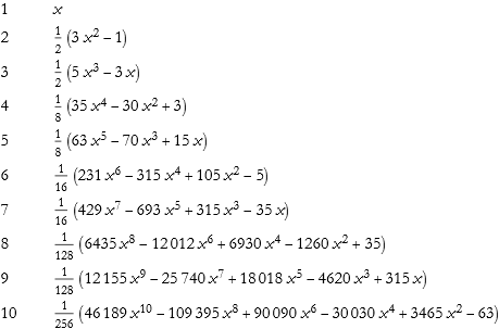
Here we produce a list of the first ten Legendre polynomials symbolically.
![]()
We can make a plot of these ten over a real domain.
![]()
Here is a plot over the complex domain.
![]()
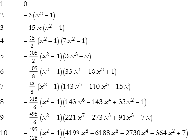
Here we produce a list of the first ten second-order associated Legendre polynomials symbolically.
![]()
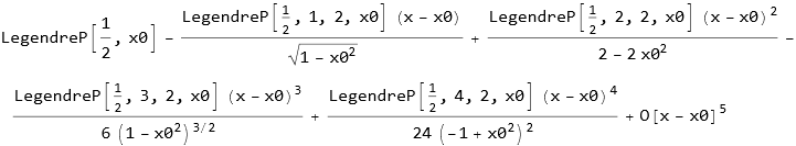
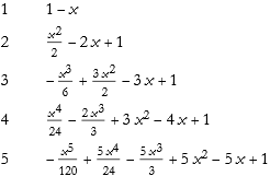
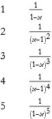
Here is the general series expansion.
![]()
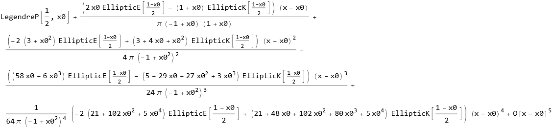
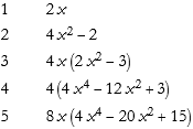
We can expand some of the Legendre terms.
![]()
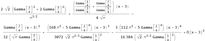
We can specify ![]() .
.
![]()
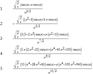
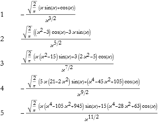
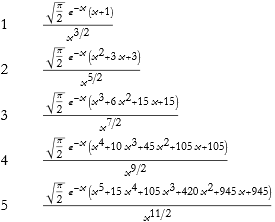
We can produce the asymptotic expansion at infinity.
![]()
![]()
As an exercise work through the documentation on LegendreP and create some examples.
Bessel Functions
Bessel functions are solutions of the Bessel equation,
![]()
(5.11)
We can get a table of the first five Bessel functions of the first kind.
![]()
Here is the plot of these functions.
![]()
We can get a table of the first five modified Bessel functions of the first kind.
![]()
Here is the plot of these functions.
![]()
![]()
We can get a table of the first five Bessel functions of the second kind.
![]()
Here is the plot of these functions.
![]()
We can get a table of the first five modified Bessel functions of the Second kind.
![]()
Here is the plot of these functions.
![]()
As an exercise work through the write-up for BesselJ, BesselI, BesselY, and BesselK and work through some examples. Look up related Bessel and Hankel functions.
Hermite Polynomials
Hermite polynomials are solutions of the equation
![]()
(5.12)
We can get a table of the first five Hermite polynomials.
![]()
Here is the plot of these functions.
![]()
Here we see the fractional Hermite polynomial on the complex plane.
![]()
(This takes a fairly long time to finish).
As an exercise read through the write up on HermiteH and work through some examples.
Laguerre Polynomials
Laguerre polynomials are solutions of the differential equation,
![]()
(5.13)
The default Laguerre polynomial, symbolized ![]() assumes a=0, otherwise we write
assumes a=0, otherwise we write ![]() and call it an associated Laguerre polynomial.
and call it an associated Laguerre polynomial.
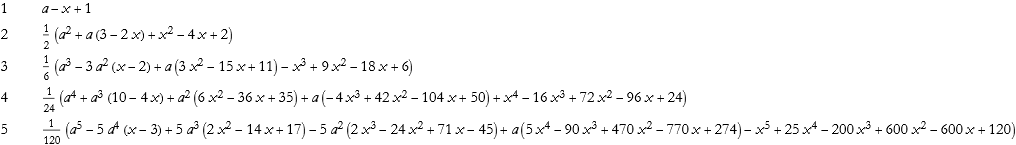
Here we write the first five polynomials.
![]()
Here is the plot of these functions.
![]()
Here we write the first five associated Laguerre polynomials.
![]()
Here is the plot of these polynomials assuming a=5.
![]()
Here is the plot of the polynomial over the complex plane.
![]()
As an exercise read through the documentation for LaguerreL and work some examples.
Chebyshev Polynomials
Chebyshev polynomials will be the last of the classical orthogonal polynomials we will discuss in detail here. Specifically these polynomials are not the solutions of a differential equation. The Chebyshev polynomials of the first kind are of the form
![]()
(5.14)
At first sight this does not appear to be a polynomial. If we apply trigonometric identities this can be converted. For example, if we choose n=2, then we can write the double angle formula
![]()
(5.15)
Using the notation in (5.14) we write, where we replace cos(x) with x,
![]()
(5.16)
Here we write the first five polynomials.
![]()
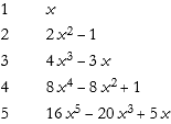
Note that the second entry is the one we derived above. Here is the plot of these functions.
![]()
Here is the plot on the complex plane.
![]()
Chebyshev polynomials of the second kind are similarly based,
![]()
(5.17)
Here we write the first five polynomials.
![]()
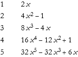
Here is the plot of these functions.
![]()
Here is the plot on the complex plane.
![]()
As an exercise work through the documentation for ChebyshevT and ChebyshevU. Work several examples.
Other Orthogonal Polynomials
These are by no means the only orthogonal polynomials in Mathematica. I recommend that you read through the section Orthogonal Polynomials in the tutorial Mathematical Functions. Look up the documentation for any that interest you and work through some examples.
Hypergeometric Functions
The hypergeometric function is defined by a power series, assuming {z}<1,
![]()
(5.18)
It has been realized that a good many special functions can be written as limiting cases or specific cases of the hypergeometric function. In that sense this is a kind of generalized special function. There are thousands of identities associated with hypergeometric functions.
Here we give an example of five functions.
![]()
Here is the plot of these functions.
![]()
As an exercise explore the different hypergeometric functions in the Guide (to listed commands) covering Hypergeometric Functions. As you read through the documentation, work up your own examples.
Other Generalizations
The hypergeometric function is not the only generalization of special functions. We will consider two of them in this section.
The first generalization was first written about in 1936 by the Dutch mathematician Cornelius Meijer (1904-1974). A very large number of special functions can be defined in terms of the Meijer G function. For a list on n values of a and m values of b we can define the G function
![]()
(5.19)
assuming r∈R. If not specified we assume r=1. To input this function we write MeijerG[{{list of a from ![]() to
to ![]() },{list from
},{list from ![]() to
to ![]() }},{{list of b from
}},{{list of b from ![]() to
to ![]() },{list from
},{list from ![]() to
to ![]() }},x]. Here are some examples.
}},x]. Here are some examples.
![]()
![]()
![]()
![]()
As an exercise work through the write up for MeijerG and work some examples.
This function being so general, we might be able to write a function as a Meijer G function.
![]()
![]()
As an exercise read the write up MeijerGReduce and work up some examples.
A generalization of the Meijer G function was accomplished by the British mathematician Charles Fox (1897-1977) in 1961. The Fox H function the Mellin-Barnes integral,
![]()
(5.20)
Here the integration is along a path separating the poles of ![]() from the poles of
from the poles of ![]() . Read the details of the write-up for more details of the possibilities of the nature of this path. This is an experimental command added to version 12.3. Here are some examples of its use.
. Read the details of the write-up for more details of the possibilities of the nature of this path. This is an experimental command added to version 12.3. Here are some examples of its use.
![]()
![]()
![]()
![]()
![]()
![]()
![]()
Here we make a table of values.
![]()
| b1 = 0 | |
| b1 = 1 | |
| b1 = 2 | |
| b1 = 3 | |
| b1 = 4 | |
| b1 = 5 |
Not much to see here. Here is a plot of these.
![]()
This takes a while.
As an exercise read through the write up of FoxH and work some examples.
Elliptic Integrals and Elliptic Functions
There are a class of functions that can be defined by the integral of some rational function R
![]()
(5.21)
where y is a cubic or quartic polynomial. This class is called elliptic integrals.
We begin with the elliptic integral of the first kind on the amplitude interval -π/2<φ<π/2 for the parameter m
![]()
(5.22)
Here we plot a list of elliptic integrals of the first kind for various amplitudes.
![]()
As an exercise read through the section on Elliptic Integrals in the tutorial Mathematical Functions. Consult each command listed there and work examples on each.
Elliptic Functions may be handled the same way, go ahead and look through the documentation and come up with some of your own examples.
Mathieu Functions
The final type of special function that we will examine today is the Mathieu function. These functions are solutions of the equation
![]()
(5.23)
The Mathieu S function is odd while the Mathieu C function is even.
Here we make a table of expressions for Mathieu S.
![]()
| a = 1 | Sin[x] |
| a = 2 | |
| a = 3 | |
| a = 4 | Sin[2 x] |
| a = 5 |
Here we plot these.
![]()
Here we make a table of expressions for Mathieu C.
![]()
| a = 1 | Cos[x] |
| a = 2 | |
| a = 3 | |
| a = 4 | Cos[2 x] |
| a = 5 |
Here we plot these.
![]()
As an exercise read through the write up on Mathieu and Related Functions in the tutorial Mathematical Function. Look up each of the listed functions and work through some examples.
There are many more special functions available to Mathematica than we can cover here. Feel free to explore these fascinating functions.