Boundary-Value and Eigenvalue Problems
George E. Hrabovsky
MAST
Introduction
Last time we discussed how to solve ODE problems in Mathematica. In this lesson we will continue that theme to include methods of handling boundary-value and eigenvalue problems.
Boundary Value Problems for ODEs
We have already discussed how to handle initial-value problems. For an ODE a boundary-value problem is one where we not only have an initial-value, but some value along the boundary of your region of concern. Say that we have a general second-order homogeneous linear ODE,
![]()
(4.1)
Say that this equation vanishes at some values of x, say a and b. We write this y(a)=0 and y(b)=0. The general solution is the linear combination of coefficients and linearly independent solutions,
![]()
(4.2)
The boundary conditions impose these requirements,
![]()
(4.3)
If the determinant of these coefficients does not vanish, then the only solution is the trivial one, ![]() . If the condition
. If the condition
![]()
(4.4)
is met, then the two expressions in (4.2) are generally equivalent and one constant can be expressed in terms of the other through elimination. If the condition in (4.4) is satisfied then the second equation in (4.2) can be discarded and the first gives us ![]() . We can rewrite these as
. We can rewrite these as ![]() , and
, and ![]() . The solution (4.3) is then rewritten.
. The solution (4.3) is then rewritten.
![]()
(4.5)
If ![]() , then this leads to a trivial solution and we must rewrite the general solution
, then this leads to a trivial solution and we must rewrite the general solution
![]()
(4.6)
assuming that both ![]() and
and ![]() are not zero.
are not zero.
For symbolic solutions, this is fairly easy to include. Say we have the equation,
![]()
![]()
Let’s say that we have the same problem, but we have a boundary where we want the solution to be, say 5, and that this occurs at a grid point of say 10.
![]()

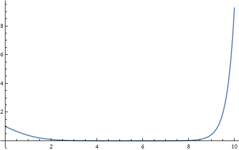
We can plot this curve.
![]()

Read through the section Initial and Boundary Value Problems in the tutorial Symbolic Differential Equation Solving. Play with some examples.
We can also apply this to NDSolve.
![]()
![]()
![]()
This might not be accurate, so let’s plot it and compare it to the symbolic case.
![]()

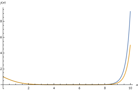
This looks good, so let’s see them both on the same plot.
![]()

We can see an inaccuracy form in the numerical solution at higher values of x. Is there a way to make this more accurate? We shall see.
Shooting Method
A common method for increasing the accuracy of BV problems is called the Shooting Method. It works like this, say we have a boundary-value problem,
![]()
(4.7)
we can write a side condition
![]()
(4.8)
where ![]() . The shooting method attempts to find initial conditions of the form
. The shooting method attempts to find initial conditions of the form ![]() so that (4.8) is satisfied. After writing g we then use some implementation of FindRoot to find c.
so that (4.8) is satisfied. After writing g we then use some implementation of FindRoot to find c.
Returning to our example. We need an intermediate expression for the initial derivative.
![]()
![]()
We now continue with our solution.
![]()
![]()
![]()
We can plot this the same way we did before.
![]()
![]()
We see no difference.
We can plot the error.
![]()
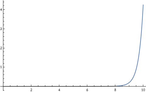
Let's see what happens if we change the method of finding the root.

![]()
![]()
No difference. We need to look at another method.
So, should we not use the Shooting Method? Let’s examine a few more cases before we pass judgement. We know that the equation we have been studying is in terms of Airy functions, so maybe that is the problem. How about an inhomogeneous linear equation?
Here we get the general solution.
![]()
![]()
What happens when we fix the boundary values at x=0 and x=1 to be y(0)=y(1)=1?
![]()

We can plot this solution.
![]()
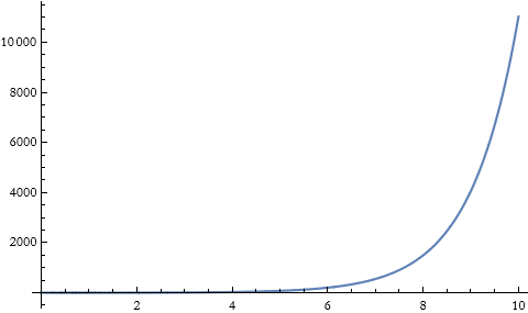
Let’s try this out with NDSolve.
![]()
![]()
Let’s plot this alongside the analytical solution.
![]()
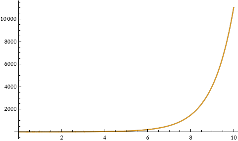
Pretty good.
In fact, you will find that the Shooting Method is pretty good in general.
Unlike IVPs, there is no theorem telling us that any solution exists, nor that such a solution is unique, for any particular BVP. So how do we know anything in general? If we look at the general solution we see a term involving ![]() . This term vanishes whenever x={0, 2 π, ...}. What happens when we try to solve for those values?
. This term vanishes whenever x={0, 2 π, ...}. What happens when we try to solve for those values?
![]()
![]()
![]()
No solution is returned.
As an exercise go ahead and work through Advanced Numerical Differential Equation Solving in the Wolfram Language tutorial, specifically the section on Boundary Value Problems and the subsection Shooting Method. Come up with some of your own examples.
The Chasing Method
There are some other methods for handling BVPs. The next one is called the chasing method, first proposed in 1965. To use this Mathematica establishes a set of auxiliary conditions that are then solved to determine initial conditions at some boundary. Once this is done, then NDSolve proceeds as normal.
![]()
![]()
![]()
We can plot the solutions.
![]()
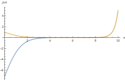
As the warning suggested the initial conditions are a problem, but starting at x=5 the previous problems disappear. We can try to increase the precision, to see if that helps.
![]()
![]()
![]()
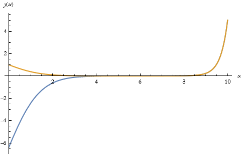
We are left with the problem of solving this equation, and as things stand we cannot do it. The shooting method is good up to x=4, then the chasing method works.
It might be interesting to see if we could use a WhenEvent option to switch from the shooting method to the chasing method.
As an exercise go ahead and work through Advanced Numerical Differential Equation Solving in the Wolfram Language tutorial, specifically the section on Boundary Value Problems and the subsection Chasing Method. Come up with some of your own examples.
Eigenfunction Expansions
It is entirely possible to go through a first course on differential equations without ever getting to the topic of eigenvalue problems. Because of this I will spend a little more time on it. Often we have an ODE similar to (4.1) where one or both of the coefficients ![]() and
and ![]() depend on a parameter λ. In these cases the determinant in (4.4) may vanish for specific values of λ. For each such value of λ there will be a solution of the form (4.5). The values of λ that produce nontrivial solutions are called eigenvalues and the corresponding solutions are called eigenfunctions. In general these types of problems are called eigenvalue problems.
depend on a parameter λ. In these cases the determinant in (4.4) may vanish for specific values of λ. For each such value of λ there will be a solution of the form (4.5). The values of λ that produce nontrivial solutions are called eigenvalues and the corresponding solutions are called eigenfunctions. In general these types of problems are called eigenvalue problems.
If we can write the equation in this form,
![]()
(4.9)
you can write the operator
![]()
(4.10)
Then (4.9) becomes
![]()
(4.11)
where g and h constitute boundary conditions, we call this type of eigenvalue problem a Strum-Liouville problem.
We can use DSolve on this kind of problem.
![]()
![]()
Here is a formal parameter that has no specified value. We can make a table of the first, say, six eigenfunctions assuming the constant of integration to be 1 and using the replace repeated command (//.).
![]()
![]()
We can plot these.
![]()
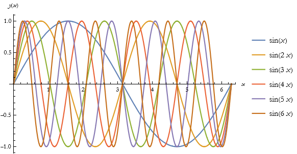
As an exercise read through the part of Scope under DSolve that discusses Sturm-Liouville Problems. Work up some examples.
Green’s Functions Solutions
There is another kind of problem, where a system responds to an impulsive type of Dirac delta. If we define a differential operator we might be able to establish a solution based on a function that satisfies homogeneous boundary conditions. If we have the operator L(G(x,y))=δ(x-y), we might be able to find G. If we can write L(h(x))=f(x) with homogeneous boundary conditions we might be able to find a specific solution by applying the convolution integral
![]()
(4.12)
If we have the initial-value problem.
![]()

We can plot this for various values of y.
![]()
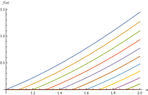
Here we have a Dirichlet-type boundary value problem.
![]()

We can plot this for various values of y.
![]()
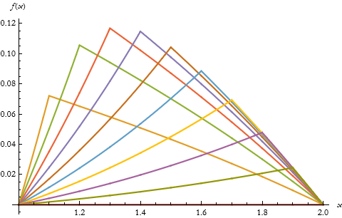
Here we have a Neumann-type boundary value problem.
![]()

We can plot this for various values of y.
![]()
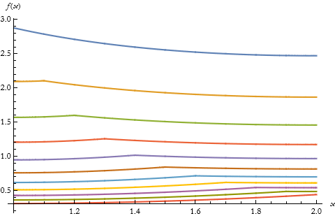
Here we have a Robin-type boundary value problem.
![]()

We can plot this for various values of y.
![]()
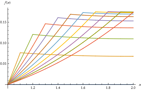
We will see more about Green’s functions in future lessons.
As an exercise, read through the documentation for GreenFunction and note particularly the ODEs section under Scope.