Ordinary Differential Equations
George E. Hrabovsky
MAST
Introduction
I trust that everyone taking this course knows what a ordinary differential equation (ODE) is. This is not the place for an introduction. I am going to proceed on the assumption that you have all encountered ordinary differential equations and have solved them in the past. What this lesson will cover is a systematic discussion of how to solve these equations using Mathematica. The chief advantages of using Mathematica are that you can solve a huge number of ODEs symbolically, you can merge numerical and symbolic solution methods, and the development time for coding is fractional as compared to other systems. If you need a quick refresher on the topic of ODEs, there is usually a pretty good survey chapter in any good mathematical methods book.
DSolve
Mathematica has a command that is designed to provide a symbolic solution to a differential equation. It can be used for ODEs and partial differential equations (PDEs), integral equations, and differential-algebraic equations (DAEs). Say we have an ordinary differential equation,
![]()
(3.1)
Solving this by hand requires us to recognize that the equation satisfies a differential operator of the form
![]()
(3.2)
We next need to recognize that this operator has equal powers of x and orders of D in each term. We need to think of an ansatz to continue, we choose ![]() , where we rewrite the equation,
, where we rewrite the equation,
![]()
(3.3)
This implies
![]()
(3.4)
We solve for a and find that a=(1,2). Thus the general solution is ![]() . Let’s see how DSolve does.
. Let’s see how DSolve does.
![]()
![]()
![]()
![]()
How do we know if this is a solution? We can plug it into the original equation and make sure it is satisfied. To do this construct each of the terms using the solution.
![]()
![]()
If we solved this using DSolveValue, we would not need the part, [[]], specification.
![]()
![]()
![]()
![]()
We then construct the equation.
![]()
![]()
So this solution satisfies (3.1).
Linear ODEs
One class of common ODEs is the linear ODE. DSolve handles these quite well. For example, here is an exponential ODE.
![]()
![]()
If we specify an initial-value of y this becomes an initial-value problem (IVP).
![]()
![]()
Inhomogeneous equations utilize the Method of Variation of Parameters or the Method of Undetermined Coefficients by default (Mathematica chooses which one to use).
![]()
![]()
Note the two parts of the solution. The second part is the general solution of the homogeneous equation.
![]()
![]()
The first part of the result in sol3 is a particular solution of the inhomogeneous equation. We can get a list of these by varying the parameters.
![]()
We can plot these.
![]()
As an exercise read the documentation for DSolve noting specifically Basic Examples and both Basic Uses and Linear Differential Equations under Scope. Work your own examples based on your reading.
Read the tutorial Symbolic Differential Equation Solving with specific reference to the sections Introduction to Differential Equation Solving with DSolve, Classification of Differential Equations, and under ODEs the subsections Overview of ODEs, First-Order ODEs, Linear Second-Order ODEs, and Higher-Order ODEs. Here you will encounter most of the kinds of linear ODEs encountered in a standard course.
Nonlinear ODEs
Mathematica is also capable of solving nonlinear ODEs. We begin with a classic Riccati equation.
![]()
Its solution is then.
![]()
![]()
Here is a second-order nonlinear ODE.
![]()
![]()
Sometimes the solution requires inverse functions.
![]()
![]()
![]()
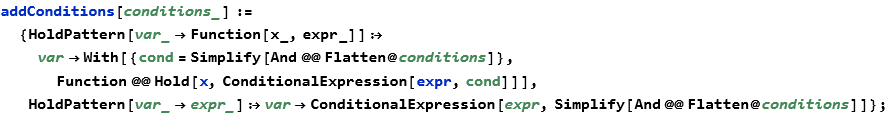
We begin by adding a set of conditions that constitute a solution for DSolve, in other words we convert a solution from DSolve into a set of conditions. This will give us a result similar to Reduce.
Here we attempt to use the command Internal`InheritedBlock.
![]()
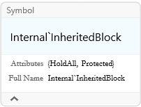
There is no advice on what it is or how to use it in the system. It is similar to Block, however one difference is that the function itself is changed locally, but not globally. Here, inside of our InheritedBlock we unprotect Solve and change it so that it uses Reduce. DSolve internally calls to Solve, so this may be a way to allow us to get results similar to Reduce.
We will also use the undocumented Internal`WithLocalSettings. This command allows to perform a cleanup so that things do not become jumbled. Specifically this applies preprocessing, then code, and then postprocessing where the postprocessing takes place before returning from aborts or similar jumps.
This method of solving the ODE can take a very long time, if it works. Be sure to copy your ODE into the expression sol= below.
![]()
![]()
![]()
![]()
![]()
![]()
![]()
![]()
![]()
![]()

![]()
![]()
![]()
![]()
![]()
![]()
![]()
![]()
![]()
![]()
![]()
![]()
![]()
These are not error messages or warnings, they just tell you that something is on or off.
![]()
![]()
![]()
![]()
![]()
![]()
![]()

![]()
![]()
![]()
![]()
![]()
![]()
![]()
![]()
![]()
![]()
![]()
![]()
![]()
This code is adapted from the work of the user Michael E2 on the Mathematica Stack Exchange.
As an exercise read the documentation for DSolve noting specifically nonlinear Differential Equations under Scope. Work your own examples based on your reading.
Read the tutorial Symbolic Differential Equation Solving with specific reference to the subsections under ODEs, Nonlinear Second-Order ODEs.
Systems of ODEs
We begin with a simple diagonal system
![]()
![]()
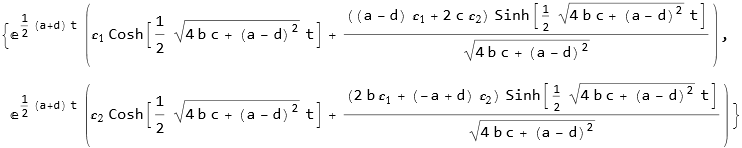
We can solve an inhomogeneous system having constant coefficients.
![]()
![]()
![]()
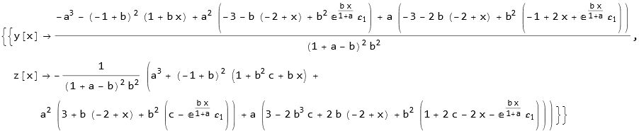
Here we have a linear system having rational coefficients.
![]()

Here we have a nonlinear system.
![]()
![]()
![]()
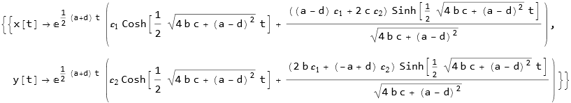
We can also perform DSolve on vector equations. Here we define a matrix and a vector function of a variable.
![]()
![]()
Not every element of the system needs to be a differential equation.
![]()
Such a system is called a differential-algebraic equation (DAE).
As an exercise read the documentation for DSolve noting specifically Systems of Differential Equations and Differential-Algebraic Equations under Scope. Work your own examples based on your reading.
Read the tutorial Symbolic Differential Equation Solving with specific reference to the subsection under ODEs, Systems of ODEs. Then read the section on DAEs.
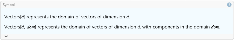
Using Symbolic Vectors and Matrices
Beginning with version 9 in 2012, a new way was introduced to abstractly represent of vectors in a specified number of dimensions. This is the Vectors command.
![]()
We can thus declare a symbol, or collection of symbols, to be a vector.
![]()
![]()
Note the assumption that the domain is the complex numbers. We can, assign this, too.
![]()
![]()
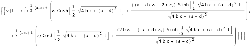
Beginning in version 13 a new type of specification in ODEs can be made. We can state that a dependent variable is an abstract vector. For example, say in sol10 above we did not specify the components of the vector V[t]. We can rename it v[t] here.
![]()
We can use DSolveValue to get the formulas without the transformation rules.
![]()
Delay Equations
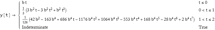
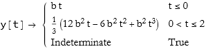
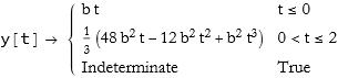
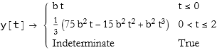
A delay-type differential equation is one where the time-derivative at some time is written in terms of the function at earlier times. In general, if our function is ![]() where we define
where we define ![]() , then the equation has the form,
, then the equation has the form,
![]()
(3.5)
We can specify this condition using the condition symbol /;.
![]()
| 1 |
|
|
| 2 |
|
|
| 3 |
|
|
| 4 |
|
|
| 5 |
|
As an exercise read the documentation for DSolve noting specifically Delay Differential Equations under Scope. Work your own examples based on your reading.
Read the tutorial Symbolic Differential Equation Solving with specific reference to the subsection under Working with DSolve. Play with some of your own examples.
NDSolve
It is inevitable that you will encounter a situation where you cannot solve an equation analytically. In such cases you will need to solve the differential equation numerically. It is used in a manner very much like DSolve, except you must specify all parameters, constants, initial-values, and boundary values. The result of any NDSolve is an interpolating function that captures the behavior of the numerical solution. It is important to realize that you should not extend the interpolating function beyond the parameters of the case that you solved. For example, if you numerically solve an equation for values of t from 0 to 25, do not expect the interpolating function to be accurate if you set t to be 100.
For example, say we have the equation and its initial condition to solve.
![]()
![]()
We can plot this equation.
![]()
We can also plot its phase portrait.
![]()
Of course, if we solve a second-order equation we need a system of two initial values.
![]()
Here we see this plot.
![]()
We can even zoom in, if we suspect small oscillations.
![]()
We can even apply it to systems of ODEs.
![]()
![]()
We can plot the dynamics of this system.
![]()
Read the documentation for the NDSolve command, specifically Basic Examples and Ordinary Differential Equations under Scope. Develop some examples and play with them.
Read the Introduction to the tutorial Advanced Numerical Differential Equation Solving in the Wolfram Language, make up some examples and play with them.
NDSolve Methods for ODEs
Unless you state otherwise, Mathematica will choose what it considers to be the appropriate solution method for your problem, but it will not tell you what it did. As with many of the commands in Mathematica, you can choose the method to use. Unlike many, there is extensive documentation of these methods in the Advanced Numerical Differential Equation Solving in the Wolfram Language tutorial. I will show off a few of these methods below.
Every course in numerical methods talks about the Euler method. It was one of the first methods and it is easy to implement. It is not the most accurate, and as we will see, it can lead to instabilities. It is an explicit method to integrate an evolution equation, thus we call it a time integration scheme. What we are doing is discretizing the time into a sequence of points and integrating at each point. Here we apply the Euler method to the harmonic oscillator problem.
![]()
We can plot the InterpolatingFunction.
![]()
One way to improve accuracy is to reduce the initial step size.
![]()
![]()
![]()
Note that this causes an increase in the amplitude of oscillation. We can see this on a phase plot.
![]()
This is what I meant earlier about instability. We can improve this by using the explicit midpoint method, often called the improved Euler method.
![]()
![]()
![]()
We have gotten a warning. It seems that we need to increase the number of steps to cover our domain.
![]()

![]()

Within the domain of interest the stability problem seems to have been solved. Here is the phase plot.
![]()
There are many more accurate methods. Here is an explicit Runge-Kutta method.
![]()
![]()
Here is the plot.
![]()
Read the documentation for NDSolve with particular reference to Details and Options, and Options>Methods. Work up some examples of your own and play with them.
Read the section of the tutorial Advanced Numerical Differential Equation Solving in the Wolfram Language ODE Integration Methods and play with some examples.
Stability and Stiffness
We have mentioned stability and even seen an example of instability. What follows is based on the online documentation.
What is stability? Let's say that we have an initial-value problem characterized by the equation
![]()
(3.6)
with the conditions ![]() and
and ![]() . We then apply the Dahlquist test equation
. We then apply the Dahlquist test equation
![]()
(3.7)
where λ∈C and Re(λ)<0. This is named after the Swedish mathematician Germund Dahlquist (1925-2005), who made significant progress in the theory of numerical analysis. We can write our numerical solution in the form
![]()
(3.8)
where, for some step size h,
![]()
(3.9)
and r(z) is a rational function representing stability. That being the case there is a region,
![]()
(3.10)
that we can call the boundary of absolute stability.
For a more concrete example we can look at the explicit Euler method described by,
![]()
(3.11)
Applying this to (3.8) we can see that
![]()
(3.12)
To continue with this we need to load the Function Approximations package.
![]()
We then examine an OrderStarPlot.
![]()
![]()
The shaded region represents instability. If we look to where the boundary of the white region intersections the negative axis, we call this the linear stability boundary (LSB). For this method we see this value is -2.
For the eigenvalue λ=-1 we need a step size such that h<2. Not hard to do. On the other hand, say we want ![]() , then we require a step size where
, then we require a step size where ![]() , very tough to do.
, very tough to do.
When you attempt to numerically solve a problem that has instabilities, we call that stiffness. Even if the point you are concerned with might be stable, if there are nearby points that are not then the problem is stiff. What is the problem? Stiff problems take longer for non-stiff methods to compute. It is an issue of the efficiency of computation. If you do not care how long your system takes to solve the problem, then you don’t have to worry about it. On the other hand, if time is a concern (say you are trying to develop a numerical forecast of the weather before the tornado occurs) then you will need some sort of stiffness handling. Most explicit methods in Mathematica have the ability to perform a StiffnessTest to allow for this possibility.
To illustrate, we return to an example from above.
![]()
![]()
Note that this has taken care of the instability of the method.
![]()
Read the section of the tutorial Advanced Numerical Differential Equation Solving in the Wolfram Language ODE Integration Methods and play with some examples.
There is an extensive discussion of this on the Mathematica Stack Exchange at the website:
https://mathematica.stackexchange.com/questions/39028/understanding-ndsolvendsz/237989#237989
Events
Sometimes we need to consider changes to the state of a system that are conditional in some way. For example, if we drop a ball and it hits the ground, it most likely will bounce. How do we capture that in a model? We use the WhenEvent[] command. For example, if we start with the equation of motion under the action of the acceleration due to gravity we write it this way, with initial conditions. We also assume that the ball bouncing absorbs 20% of the force with each bounce.
![]()
We can plot this
![]()
Go ahead and read the documentation for the WhenEvent command. Pay particular attention to the Details and Options, and then to Applications. Make up some examples and play with them.
A More Traditional Numerical Approach
There are those people who are, for one reason or another, wanting to do things the old fashioned way. In a later lesson we will explore more deeply the ideas of finite differences. Here we will give an overview of how to duplicate the results of older, tried and true, methods. We begin with a differential equation and an initial condition.
![]()
![]()
We apply the DifferenceQuotient command to make this into a difference equation.
![]()
![]()
We have already seen the solution of this in ivp1. We can use DSolveValue to get the solution as a formula.
![]()
![]()
We use RSolveValue to get the formula to solve the difference equation.
![]()
![]()
We can compare the plots of these for any case where we assign a value of a.
![]()
We will explore this more in a later lesson. I will note that as of version 13 RSolve is now able to solve all linear systems with polynomial coefficients.