Data Analysis and Fitting

George E. Hrabovsky

MAST

Introduction

In the last lesson we discussed how to use some basic mathematical techniques in Mathematica that are relevant to computational science. In this lesson we will use those techniques as a foundation and study how to use a computer to analyze data, specifically how to use Mathematica to analyze data. This is a huge subject, worthy of a course in itself, so we will only study those techniques that lead to other computational techniques that we can use to make models down the road.

What we mean by data is a set of results distributed with respect to some dependent variable whose dependency we may not already know. Say for example that we have a set of n values, each indexed from 1 to n, . We think of these values as the result of some unknown function, f, of values—also indexed from 1 to n, . We can write this,

(2.1)

The task of data analysis is to try to figure out what f is by examining the data. Such a result is often called an empirical formula. Many physical laws begin as this kind of empirical formula.

One question is, “Can we apply these techniques to computational modeling?” The answer is yes. Say you have a numerical result that constitutes a list of ordered pairs. Using these techniques you might estimate an empirical formula to describe them.

Matrix Operations

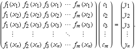
One way of thinking about data is as a list. A list is little more than matrix. So we can think of a set of data as a kind of matrix. Even if it is only a column or row matrix. We can give an example, let’s say that we have determined that our function is a polynomial,

(2.2)

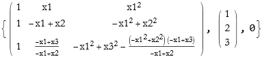
To truly solve this system for n values of x, we can write this as a matrix applied to a vector (the coefficients) to find the solution vector.

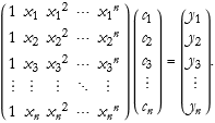
(2.3)

As an exercise, rewrite this for arbitrary functions of , where we can assume arbitrary fitting functions for each value.

How do we solve this in Mathematica?

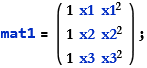
We can write the solution for the coefficients in order.

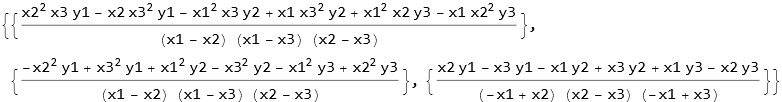
What we call sol1 is what we had earlier called cvec,  the first solution is , the second , and the third .

We can rename this matrix mat1 as S. We can call cvec by the symbol c, and yvec as y. We then rewrite (2.3),

(2.4)

Matrix multiplication is accomplished by using the dot symbol.

Matrix transpose is also easily done.

Determinants are also easily found.

It is often useful to factor a square matrix into products of matrices determined by the eigenvalues of the square matrix. This is called a decomposition. There are many such different types of decomposition.

The first method we use decomposes the matrix into the product of a unitary matrix called Q and an upper triangular matrix called R, we call this the QR Decomposition. This only works for numerical matrices.

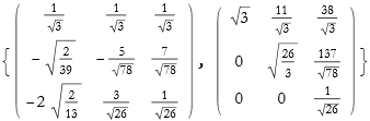
The first matrix is Q, the second R.

Another decomposition converts the matrix into a product of lower and upper triangular matrices, called the LU decomposition. In Mathematica the first result is the LU decomposition, the second is a vector that specifies the rows for pivoting, and the third result is the condition number for a numerical matrix.

A decomposition resulting in a conjugate transpose and a diagonal matrix is called the singular value decomposition, SVD.

These three matrices may be labeled u (an n×n orthogonal matrix), v (an n×m diagonal matrix), and v (an m×m orthogonal matrix). The decomposition is then,

(2.5)

When we solve a matrix equation we invert the matrix. This is fine so long as the matrix is not singular. If the determinant of the matrix is zero, then it is said to be singular. A singular matrix cannot be inverted. A robust method for finding the pseudoinverse is called the Moore-Penrose method, and this even applies to singular matrices.

Since mat2 is nonsingular the inverse can be found.

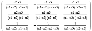
Exact Fitting

If we have perfect information about the data points, then we can fit the data points exactly. In that case we write an equation similar to (2.4), we can solve for the coefficients,

(2.6)

By applying the inverse of the transformation matrix to the vector of the data we want to fit.

For example, we have a set of data points.

We can see these points.

We have six points, so let’s try to fit a set of polynomials to the points.

We can see which of these is the best fit.

We can see that the 5th fit is the best, connecting every point.

Approximate Fitting

It is almost impossible to have exact information about measured data. All measurements have errors. Sometimes due to noise, sometimes due to systematic uncertainties. So how do we deal with this eventuality? We can use the same sort of method, though with a different formulation. In this case we still have the n data points, but with m terms.

(2.7)

The solution will be of the form,

(2.8)

Here the S matrix is an m×n rectangular matrix instead of the square matrix we had before. The problem is that we cannot invert such a matrix. Of course, we are left with the fact that we cannot produce an exact fit to this data. Instead we need to discover the function that gives the best fit of the data. We call these functions basis functions.

This best fit is best determined by minimizing the distance between a data point and the curve of the fitted function. Another way to look at this allows us to write a data point as an ordered pair , the corresponding function value is . The square of the distance between these is then . We call the sum of these distances the residual. We denote this with the Greek letter χ.

(2.9)

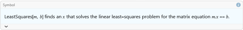
The smaller this number is, the better the fit. We call this the linear least squares. More generally, given some matrix m and some argument b (this can be a vector or a matrix), we have the matrix equation

(2.10)

The method of least squares finds the value for x that minimizes the norm {|m x - b|}. In Mathematica we can use the LeastSquares command.

We can check this.

This function has existed in Mathematica since version 6, but in the new release (version 13) you may choose one of several methods.

This is for dense or sparse matrices.

This is good for dense matrices.

This is good for dense or sparse machine number matrices.

This is good for sparse machine number matrices.

The problem of applying the least squares method to data is to discover the coefficients that minimize the residual. This is the purpose of the Moore-Penrose pseudoinverse.

If we apply the pseudoinverse to the transformation matrix by matrix multiplication we get an identity matrix. Again we have , where c is the solution of the least squares problem.

Here we see an example of this. Say we have a set of points.

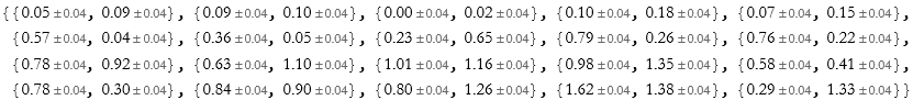
We can plot these.

We can get the data points without the uncertainties for fitting.

]

We can attempt to fit this set of data with various polynomial fits.

None of them are doing particularly well. If this were a fit to a set of models, few of them hit the error bars and none are very good. The best is the fifth-order polynomial fit.

We can try other functions.

As an exercise look up the FindFit, LeastSquares (particularly the Applications section) command. Try applying these functions to the data given above.

There is another effective way to smooth out these fits. We introduce a measure of the roughness of the residual, and we want to minimize this roughness. This roughness represents the lack of smoothness in the fitted curve. What constitutes the roughness? It can be pretty much anything in the form of the product of a matrix and the fit coefficients. One basic assumption is homogeneity. If R represents the roughness matrix and c is the coefficient vector, then we can write the homogeneity condition.

(2.11)

Here we note that R is an n r×m matrix, r being the number of specific roughness constraints. We can assume that this equation can’t be satisfied (a smooth function has no roughness and can’t fit the data). On the other hand we seek to minimize the square of the roughness, along similar lines to the linear least squares method. We expect that this would look something like . We call this regularization.We then construct a compound matrix system. If we adopt the symbol λ as a control of the weight of the smoothing, then first n rows are S, the next n r rows are λ R. Thus we rewrite (2.10)

(2.12)

We can solve this for c, thus finding the set of coefficients that fits the best. The total residual of all of this

(2.13)

is minimized.

A useful idea is to make the roughness function be represented by the second derivative of the function at specific points ,

(2.14)

This is equivalent to something that we could call a smoothing spline.

We can test this out. Beginning with version 12 Mathematica has the ability to perform regularization.

Here we have chosen the second-order difference to represent the second derivative roughness function. Since the vertical scale is a factor of 1, we have chosen λ to be 1.

What happens if we choose a different λ?

There is a little bit of variance, but not too much.

We can apply this regularization to solving equations for rough functions, too.

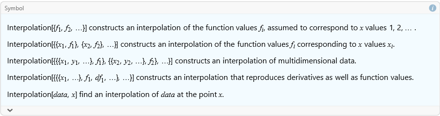
Interpolation

It is possible to approximate the function describing a set of data by defining a smooth curve that connects all of its points. This is called interpolation. In MMA we use the Interpolation command.

For example.

We can see a plot of this.

We can use the interpolated function just like it is any kind of function, though it may not be possible to get a formula for it. It is an entirely numerical approximation of a function.

Image Reconstruction

If we were to shoot a beam of x-rays through an object we could measure the attenuation of the beam and get an estimate of the density through the material along the path of the beam. If we do this many times along chords in a plane section of the material, then we can integrate our density estimates to reconstruct the material along that plane section. This is a process called x-ray tomography.

Given a set of coefficients and a set of basis functions we can represent the density in this form,

(2.15)

The basis functions can be as simple as a set of pixels covering the plane area. They can be very complicated with the requirement of a second index for a second dimension in the plane.

Each measurement chord passes through the basis functions. Thus, for each set of coefficients we get a chordal value of our measurement along each line of sight ,

(2.16)

This allows us to write our fitting problem in a standard form.

(2.17)

We can solve this problem by the pseudoinverse so long as it is overdetermined by a large number of basis functions.

In practice this is almost never the case. For a variety of reasons the system is usually underdetermined (there might not be enough independent chordal measurements to determine the density of each pixel). Why? The noise inherent in the chordal measurements is amplified by the inversion process, so you get unwanted artifacts.

The solution is smoothing by regularization. The roughness function is a Laplacian that is evaluated at each pixel.