Monitoring Numerical Solutions and Building Your Own Numerical Solutions

George E. Hrabovsky

MAST

Introduction

So far we have been using what amount to a set of black box tools in Mathematica. It is, of course, possible to learn what algorithms are being implemented, but that does not mean you will understand the implementation of those algorithms. In this lesson we will begin by exploring some tools to make using these black boxes more effective. Then we will learn how to construct our own finite difference schemes. Then we will explore several methods of solving differential equations in detail: Verlet, Euler, modified Euler, Runge-Kutta, Multistep, Lax-Wendroff, and Crank-Nicholson. We will end the lesson with a discussion of how to add methods to the existing NDSolve framework.

Reap and Sow in Numerical Integration

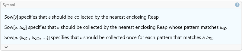
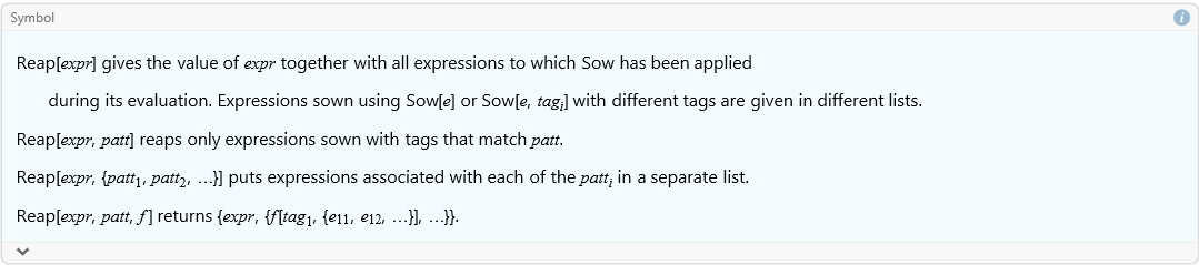
Two associated commands are Reap and Sow.

For example, we can plot the behavior of an interesting function.

We can numerically integrate this and visualize the points it is using to evaluate the numerical quadrature. We use the command EvaluationMonitor.

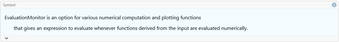
To put this another way, it will return a result any time a numerical evaluation is triggered.

This is not a very illuminating plot unless you understand how the increasing density of points demonstrates convergence, but it is a bit mysterious. Every time a numerical integration occurs it sows a result. These sowed results are collected as a list by the reap and then displayed. Here is a plot that uses the same information, but displays it along the function curve so we can better understand what is happening.

In the places where the curve is harder to integrate there are more points considered, in other words the method adapts to the difficulty of integration.

Using StepMonitor in NDSolve

So, how do we know that a solution is progressing during an NDSolve evaluation?  We will use StepMonitor for this.

We begin by creating a plot that updates automatically. This will be our monitor.

Right now this is empty. We will fill it shortly. Watch the plot change as the solution converges to a result.

Using Monitor and Progress Indicator

We can make an additional monitor using the Monitor and ProgressIndicator commands.

Here we make another plot that updates, to track the progress of our NDSolve.

Then we have our solution with the new monitor.

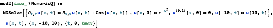
Using NumericQ

We can make our own function to solve the previous equation.

We can run this.

There may be times when this returns a result that informs you that you must use a numerical value even though you are using one. To avoid this case we add the following statement (and this can be used for any command requiring a numerical input).

We test this.

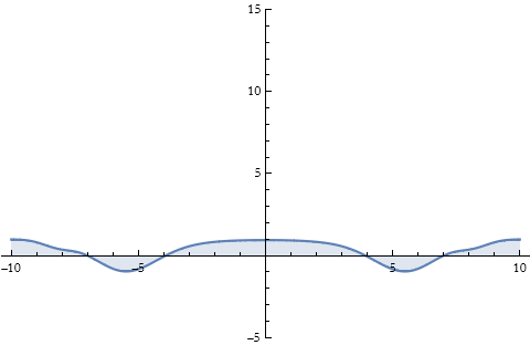
Now we can see where it becomes useful.

Using RSolve for Differences

So the traditional way of solving ODEs and PDEs on a computer is to convert the differential equation into a difference equation. This effectively turns the analytic task of integrating the ODE or PDE into solving a matrix-valued difference equation. So how do we set up such a difference equation in Mathematica? Just as there are methods of solving equations and differential equations, there is a system for difference equations called RSolve.

Let’s take a look at a linear difference equation with constant coefficients.

(12.1)

How do we solve this?

We can also use this to solve an IVP. Say we have the equation above, but with the initial conditions y(0)=1, y(1)=5, and y(2)=-1.

We can plot the real part.

The imaginary part is very small.

We can investigate what happens if time continues.

Let’s take a case that we know the form and see how to convert it to the finite-difference scheme. Take the ODE

(12.2)

with the initial condition that y(0)=1.

We try DSolve .

We can plot this..

The derivatives become difference quotients. For a forward difference representing a derivative we have.

For a second derivative, we write this.

We can write the backwards differences, too.

and the second derivative is then.

We can also use central differences (this is good for spatial derivatives).

and the second derivative is then.

To discretize our differential equation we write,

We solve this for a value of h determined by the user.

We can turn this into a function of h.

We can plot this.

We can compare them.

Our Own Explorations

Those of you who have programmed in FORTRAN, C++, Java, and the like are familiar with the idea of procedural programming as that is the style used in these languages. Procedures are executed in looping structures.

We begin by converting the diffusion equation to its finite-difference equivalent,

(12.3)

Here we have a ring divided into X cells for N time steps. Then we specify a given cell’s density by considering the ith cell for the nth time step. So we say that i extends from 0 to X, and the time extends from 0 to N. For any specific time step we will have,

(12.4)

We can determine the stability condition to be,

(12.5)

If this ratio is more than 1/2 the solution will become unstable in time. We write,

(12.6)

So how do we implement this in Mathematica?

If we have some set of initial conditions for ρ as ρ0, then we can use the above formula to get a set of the next time step of values for ρ, we can then relabel these as the new ρ0 values and continue the calculation. We have to establish the initial conditions, and I will use the procedural iterator Table[function, {iterator}] to produce this result.

Let’s say we choose the option for positions 0 to 6.

we then develop the current time step as the initial conditions, here I specify the part of the list considered by the convention list[[part of list]].

Here we have the periodic boundary conditions.

this completes the initialization step, and we have established the initial condition.

We now establish a single time step be rewriting ρ[x] to include the boundary conditions. I use the If[condition, condition is met, condition is not met] for this.

We test this.

Then we can establish a time step, here again I use Table to generate the list.

We check this.

We now construct the solution in time, using Table.

This completes the model development.

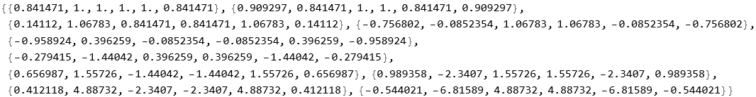
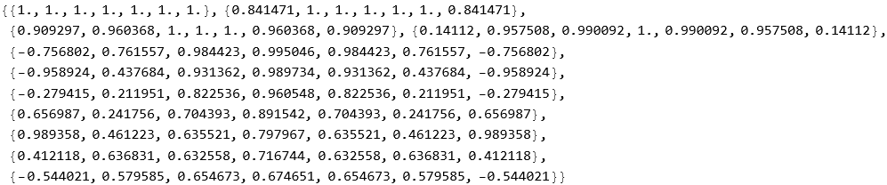
Now we need to display the results. I make a test run.

Here is the plot of these results.

This distorts and gets noisy very fast, of course we violated the stability condition with our choice of D, so lets try it again, we know from (12.5) that D≤1/4. We need to reinitialize ρ0.

Then we construct the run using the correct value for D.

This takes a long time to run and produces the result.

Compare this with the solution to the diffusion equation from lesson 10.

That looks better. This looks like the result we got from NDSolve with some additional noise. We could use a finer grid and a better difference scheme if we wanted to get more precise and more accurate. That is, however, the subject for another talk.

Another style of programming uses f(x) as the application of f to x. So we start by establishing a function in the traditional way, using the Function[body][parameter replacement] command. Here we use the notation # to represent a formal parameter.

We could write this without the Function command, but then we need an ampersand following the function statement so that Mathematica will know that the function statement is done.

We can also write these for multiple variables.

Or we can write it without the Function[] command.

We can apply a function to a list by the use of the Map[function,{list}] command.

We could also use the command line f/@.

Say we want to program the diffusion equation in functional programming. We begin with establishing the list of cells in our ring. We employ the Range[max element] to produce a list from 1 to X.

We decide we want to go from 1 to 6.

We now establish our initial conditions.

For our choice of initial conditions we have, 1 everywhere, so we just tell it to divide by itself at each location.

Now we specify the diffusion equation. Since we have periodic boundary conditions and a list we can just rotate the list right and left.

We can test this.

We now need to impose our boundary conditions. Here we are replacing the end parts with the boundary conditions using ReplacePart[list,{parts and replacements}].

We will test these.

So we construct a single step.

Let’s try it.

We can construct a table to produce our result.

We can try this.

We can plot this to see how we did.

We have gotten the same result as for procedural programming. It also took almost no time.

Another style of programming uses the symbolic nature of Mathematica to transform expressions. This is called ruled-based programming, and uses the notion of rewrite rules, this is because you rewrite an expression. This is a very different style of programming. Here we take an expression,

and we apply a transformation rule to it,

Using our example above, we begin with the initial conditions.

Then we execute it.

Then we have the diffusion equation. Here the double underscore __ following the ρ0 signifies a list.

For our example

we can include the boundary conditions.

We can test this again,

We can then produce our model.

The Verlet Method

Here we implement the Verlet method for solving the Newtonian equations of motion. If we have

(12.7)

we can assume that the solution will be . We can expand this as a Taylor series for some small time interval Δ t.

(12.8)

and

(12.9)

If we know and , and if we calculate , then we can add (12.8) and (12.9) to get,

(12.10)

The velocity is then the difference.

(12.11)

So we get a set of positions each of which is identified by (12.10) assuming we know the force. This allows us to write the acceleration as an input. If we couple that with initial position and initial velocity we are almost there. We have one subtle problem remaining, since we want this is the same thing as finding . Rewriting (12.11) we get,

(12.12)

All we need to do is calculate . This allows us to find for each subsequent time step. If we supply the acceleration function (the right-hand-side divided by mass as a function of position and time), the initial position and velocity, the size of the time step and the number of steps we can solve the equations of motion in general.

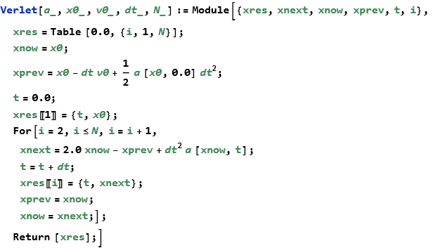
This program was presented (with some alterations) in the book by Joel Franklin, (2013), Computational Methods for Physics, Cambridge University Press. I want to like this book and it covers a lot of ground. The biggest problem with it is that the author is obviously a FORTRAN/C programmer who thinks in terms of procedural programming. There is nothing wrong with this, except that it is almost never the best way to program in Mathematica. Mathematica (and the Wolfram Language in general) allows you to program in every programming paradigm as you like (you can even shift from one to another in the same line of code without trouble). As an exercise write this again using either functional or rule-based style programming.

Euler’s Method

If we have a differential equation,

(12.13)

with the initial condition

(12.14)

then we can approximate the solution by,

(12.15)

and

(12.16)

We can write this in Mathematica.

We can test this for a simple quadratic function.

We can then make a set of data based on applying the Euler method to this function .

We can plot this .

We can compare this to the result of DSolve.

We can plot this.

This code is based on the web page

http://homepage.cem.itesm.mx/jose.luis.gomez/data/mathematica/metodos.pdf .

Improved Euler Method

Euler’s method is quite crude. There is a more accurate version that is sometimes called the improved Euler method, and sometimes it is called Heun’s method. We can borrow some notation from the last section and write,

(12.17)

We can write this in Mathematica.

This was taken from the website https://engcourses-uofa.ca/books/numericalanalysis/ordinary-differential-equations/solution-methods-for-ivps/heuns-method/ and suffers from the same procedural bias. Make no mistake, procedural programs work in Mathematica. It is just that these programs work extremely slowly as compared to the other styles of programming.

As an exercise, write this in a more efficient form.

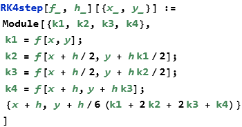
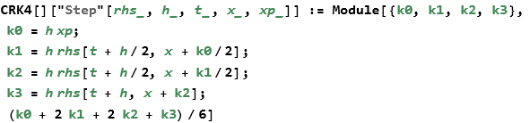
Runge-Kutta

A more advanced, but also demanding, solution method is the Runge-Kutta method. There are many different RK methods. We will look at the classic RK, or RK4 method. The method uses the equations,

(12.18)

(12.19)

(12.20)

(12.21)

(12.22)

(12.23)

We can make a single RK step.

We can then apply the NestList command to perform the solution starting at and then working through the solution.

This code is adapted from a discussion on Mathematica Stack Exchange: the web site address is:  https://mathematica.stackexchange.com/questions/220165/runge-kutta-implemented-on-mathematica . This is a great site for uncovering good style and addressing problems.

Multistep Methods

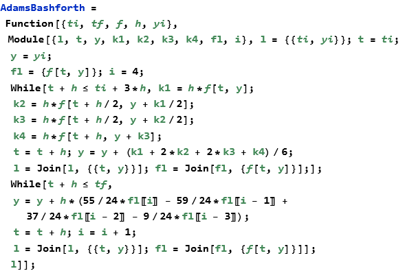
Adams Method

There are many other methods that require multiple steps in a manner similar to the RK4 method. One that is quite common in such courses is the Adams method named for the English mathematical John Couch Adams (1819-1892). Using this method we rewrite our differential equation,

(12.24)

we then approximate f(t,d(t)) by the k-degree polynomial . So, if approximates our slope function, then we require that for

(12.24)

and for

(12.25)

We solve for a and b

(12.26)

(12.27)

So we have developed a polynomial to approximate our derivative. We can think of this as a predictor step. If we then replace our slope function with our polynomial and then evaluate the direct integral we get our second step,

(12.29)

This result is called the first-order Adams-Bashforth formula, named for Adams and the English mathematician Francis Bashforth (1819-1912).

Here is an implementation from the Mathematica Stack Exchange due to a collaboration between user MarcoB and Alex Trounev.

The Backward Differentiation Method

In this method we also use a polynomial, here to approximate the solution of an IVP instead of a derivative. Here our predictor step proceeds along the same lines as (12.29),

(12.30)

here the difference is that the derivative , so we make an additional requirement,

(12.31)

We can then find (by subtracting (12.29) from (12.31) that

(12.32)

we then get the first-order backward differentiation formula.

(12.33)

This is due to the work of the English-America mathematician C. William Gear (born 1935), this work was done in the 1970s when Gear was interested in stiff equations.

The Predictor-Corrector Method

We can use the Adams method as a predictor, we can then apply a backward formula and arrive at the predictor-corrector formula,

(12.34)

(12.35)

This method has been attributed to the Finnish mathematician Evert Johannes Nyström (1895-1960).

Lax-Wendroff

What follows is due to Hungarian-born American mathematician Peter Lax (b 1926) and the American mathematician Burton Wendroff (b 1930). Their work was done in 1960. If we have the advection equation,

(12.36)

Lax and Wendroff decided that we can apply a difference formula to the right-hand side. We can rewrite the right-hand side partial derivative,

(12.37)

We can then add a term,

(12.38)

We apply differences to each term and get the Lax-Wendroff scheme for the advection equation,

(12.39)

I found no good implementations of this method, nor have I ever used it in my work. I did find a very old and clunky implementation in a very good book by Victor G. Ganzha and Evgenii V. Vorozhtsov (1996), Numerical Solutions for Partial Differential Equations Problem Solving Using Mathematica, CRC Press (a truly great book for people who want to get down and dirty in the numerical methods). This implementation is step by step and very pedagogical. As a quick dodge I then assign it as a project idea. I guarantee that if you complete such a task, people will use it.

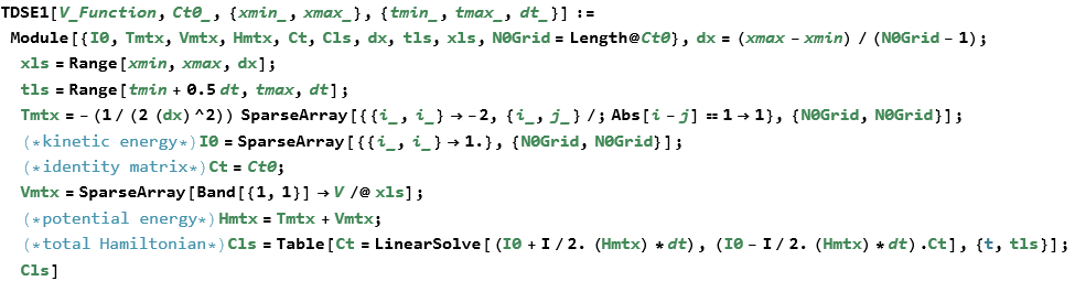
Crank-Nicolson

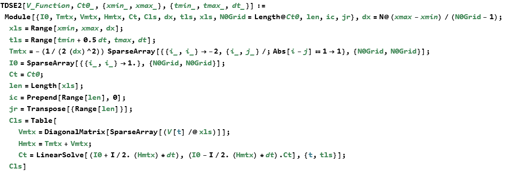
The Crank-Nicolson method was developed in 1947 by the English mathematical physicist John Crank (1916-2006) and the English mathematician and physicist Phyllis Nicolson (1917-1968). If we can write a PDE in the form,

(12.40)

then we can rewrite it

(12.41)

Here we have a solution of the one-dimensional time-independent Schrödinger equation for a position-dependent potential.

We can see the results of this.

For a time-dependent potential we have this.

Here is the result of this calculation.

This implementation was found on the Mathematica Stack Exchange as a result of a collaboration between the users xslittlegrass, Leonid Shifrin, and Jens.

Incorporating Methods into NDSolve

One nice feature is that you can write a method and incorporate it into the existing NDSolve structure.  If we adopt our RK4 method given above, we can write our steps in this way.

We can specify all of the inputs and outputs for our step function.

Of course, we can also use the actual names for these instead.

We can now specify a method allowing NDSolve to make the proper difference order for that method.

We then define the step mode, in this case we make it fixed, since the method has no step control.

So that is all we need. We try it out on the oscillator equation.

We can plot this.

Here is a second example. This time we couple our new method with a step control method called DoubleStep.

The plot here is given.

We can compare the error.

These examples are drawn, with minor variations, from the section on NDSolve Plugins in the tutorial Advanced Numerical Differential Equation Solving in Mathematica.