Hyperbolic Equations
George E. Hrabovsky
MAST
Introduction
In this lesson we examine how to solve hyperbolic equations in Mathematica. We begin with the wave equation. We study the D’Alembert solution. Then we discuss initial value problems. Then we talk about inhomogeneous wave equations. We then turn to boundary conditions and unbounded regions. We then explore how to solve the equation with Fourier and Laplace transforms. Then we turn to the telegraph equation as a generalization of the wave equation. We will then expand our discussion to problems in two- and three-spatial dimensions.
The Wave Equation
Say that we have a string of length ℓ that is fixed at both ends. Assume that there are vibrations that occur in a plane so that displacement of the vibrations is transverse to the string. If we define the amplitude of the vibration is a function of position and time, u(x,t) then the equation describing the vibrations given a wave speed for the material of the string c is
![]()
(11.1)
The right-hand side is the net force due to the tension of the string. Because we have a second time derivative we need two initial conditions.
![]()
(11.2)
Assume that c=1 and ℓ=1, then our equation will be written.
![]()
![]()
We can establish our initial conditions.
![]()
We can also write our boundary conditions.
![]()
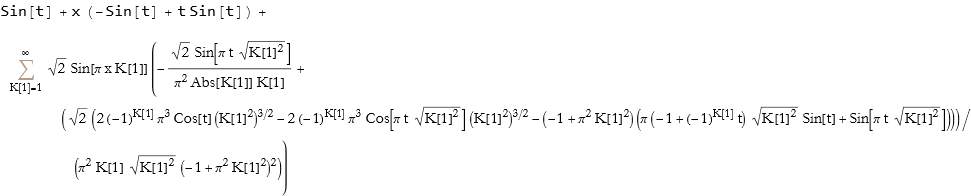
We now construct our solution.
![]()
![]()
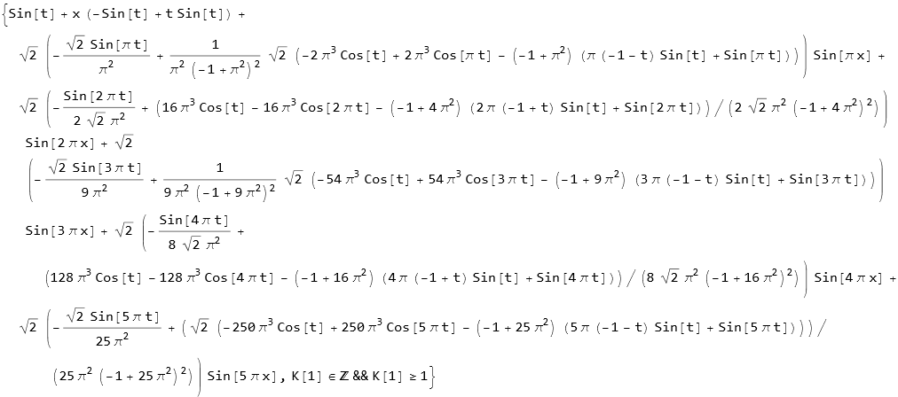
We take the first five terms.
![]()
![]()
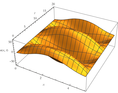
We can plot this .
![]()
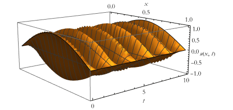
![]()
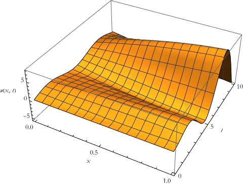
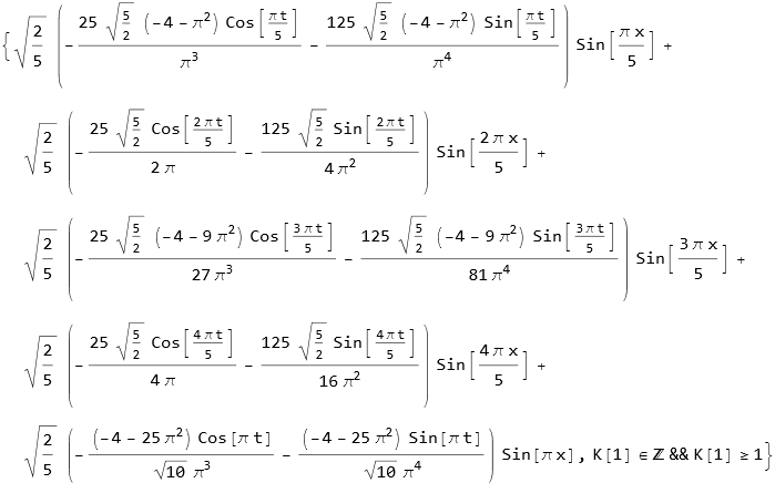
This is a very strange plot. There might be artifacts. Let’s increase the number of terms.
![]()
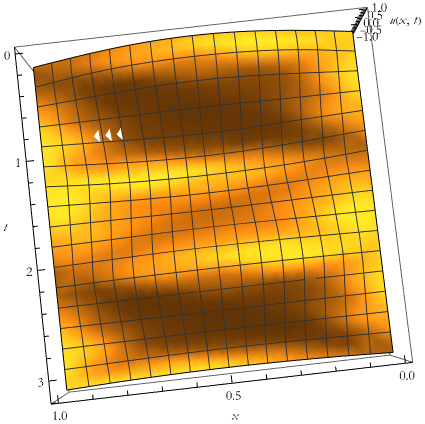
The new plot is then.
![]()
Let’s examine a specific value of t.
![]()
Let’s make an animation of this.
![]()
D’Alembert’s Solution
Given the wave equation (11.1), it is possible to introduce two new variables,
![]()
(11.3)
and
![]()
(11.4)
We can then rewrite u(x,t) as f(μ,ν). We can then rewrite the wave equation,
![]()
(11.5)
We can write this equation.
![]()
Its solution is then given.
![]()
![]()
Reversing the transformation, we get a general solution to the wave equation,
![]()
(11.6)
We can get this solution by using DSolve by first writing the general wave equation.
![]()
![]()
We can then get the solution.
![]()
![]()
So we have two characteristic functions. This is called the d’Alembert solution, after the French mathematician and physicist Jean le Rond d’Alembert (1717-1783).
IVPs
If we apply an exponential initial condition, we will see an interesting phenomena.
![]()
We then construct our solution.
![]()
| |
|
We can plot this.
![]()
This displays the characteristics well.
We can also introduce an initial condition involving piecewise defined initial data.
![]()
Now the solution looks like this.
![]()
| |
|
The solution can be plotted.
![]()
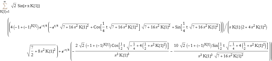
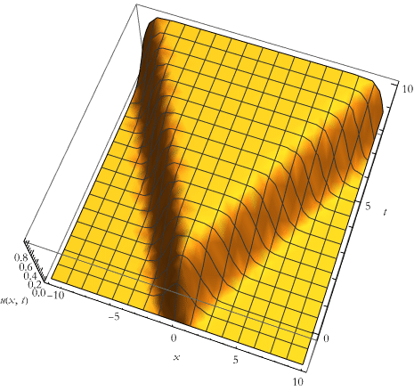
We can also examine a decaying exponential function as an initial condition.
![]()
Here we write the solution.
![]()
| |
|
Here is the plot of this solution.
![]()
The Inhomogeneous Wave Equation
An inhomogeneous version of the wave equation is of the form,
![]()
(11.7)
We write the equation.
![]()
We can write an interesting initial condition.
![]()
The solution is then.
![]()
| |
|
We can make a table of plots for various values of f.
![]()
| -1. | 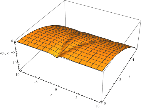 |
| -0.8 |  |
| -0.6 |  |
| -0.4 | 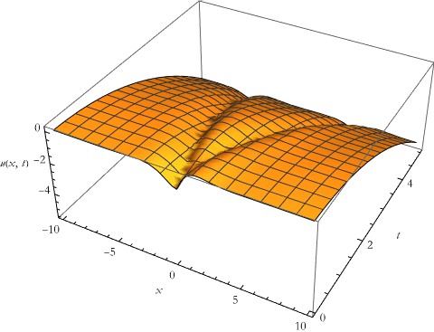 |
| -0.2 | 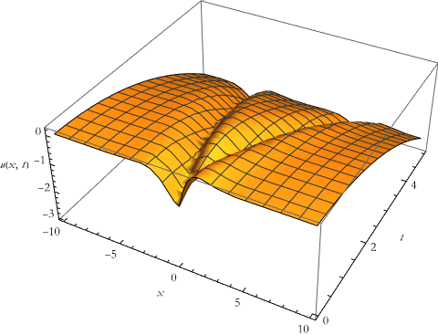 |
| 0. | 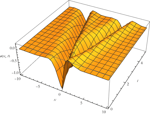 |
| 0.2 | 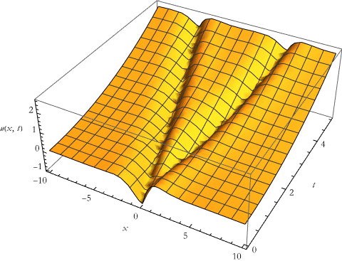 |
| 0.4 | 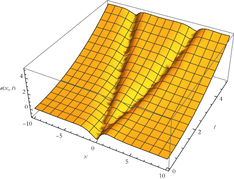 |
| 0.6 | 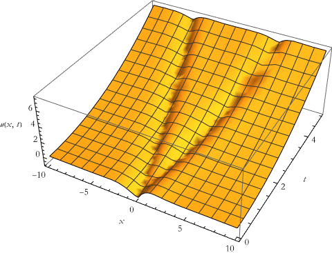 |
| 0.8 | 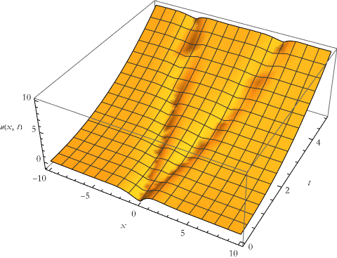 |
| 1. | 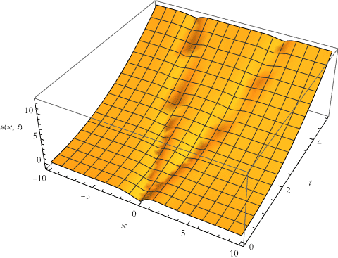 |
| 1.2 |  |
| 1.4 |  |
| 1.6 | 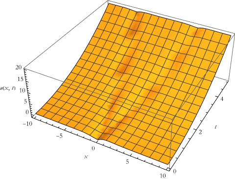 |
| 1.8 |  |
| 2. | 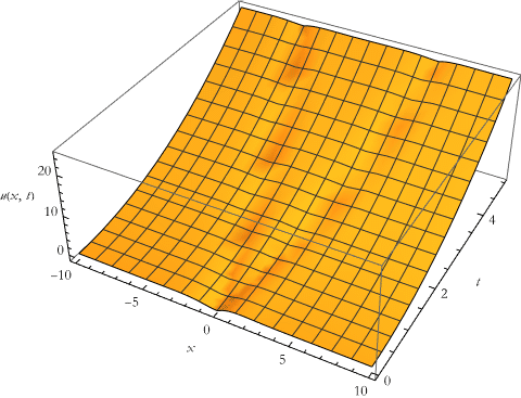 |
Boundary Conditions
Boundary conditions for this type of equation are similar to what we have covered so far. I will examine a source on a boundary, in other words an inhomogeneous boundary condition. We will use eqn1 from above.
The initial conditions are written.
![]()
The boundary conditions are then written so that a source term appears.
![]()
We then build our solution.
![]()
| |
|
We can get the first five terms of this series.
![]()
We can plot this.
![]()
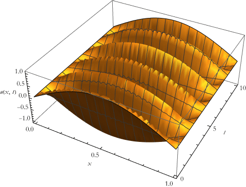
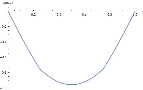
If we apply a quadratic source as an initial condition while fixing the endpoints, we use Dirichlet conditions. We write the initial conditions.
![]()
The boundary conditions establish the fixed endpoints.
![]()
We then build the solution.
![]()
![]()
We extract the first five terms.
![]()

The plot of this if then given.
![]()
If we have a quartic source, we can use Neumann conditions.
![]()
We then build the solution.
![]()
![]()
We extract the first five terms.
![]()
The plot of this if then given.
![]()
Let’s say that we have one end that is strictly controlled and we apply a force to the other end. On one end we have a Neumann condition and a Dirichlet condition while the other end is allowed to be free of any initial condition.
![]()
We then build the solution.
![]()
| |
|
We extract the first five terms.
![]()
The plot of this if then given.
![]()
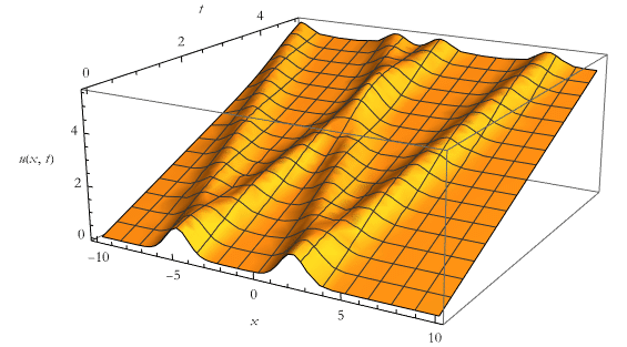
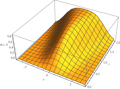
Unbounded Regions
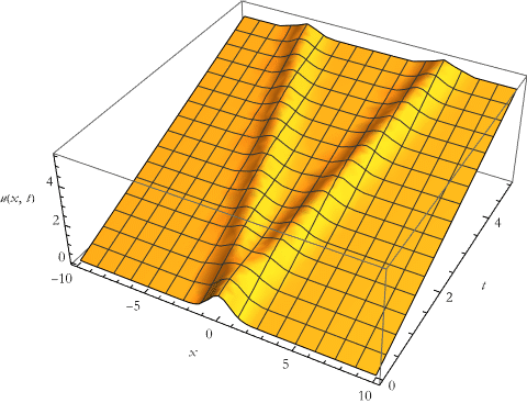
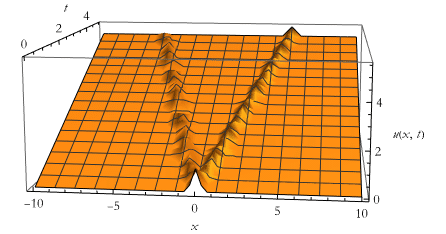
As in the previous cases we can establish unbounded regions. For example, if we extend our string to be the whole line, we would use (11.1) and the following initial and boundary conditions,
![]()
(11.8)
We can input these into Mathematica.
![]()
The solution is then calculated.
![]()
| |
|
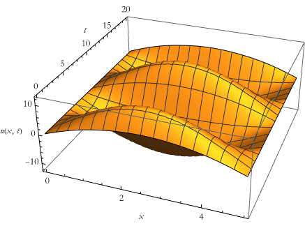
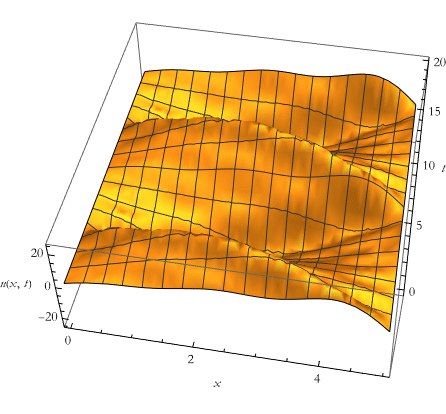
We can plot this.
![]()
We can see the detailed evolution of this wave.
![]()
The Fourier Transform Method
We can rewrite eqn1 using Fourier Transforms
![]()
![]()
We can translate this into something we can read.
![]()
![]()
Let’s adopt the initial conditions for an infinite string and Fourier transform them.
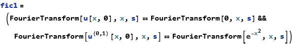
![]()
Again we make this readable.
![]()
![]()
We now have a simple differential equation for the function U. We can solve this IVP.
![]()
![]()
We transform this back to get the solution.
![]()
![]()
This is the result we got above.
Laplace Transforms
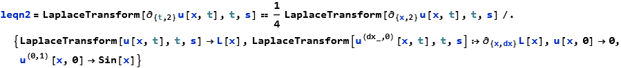
We can attempt to solve our previous equation using Laplace transforms. We begin by transforming the equation.
![]()
![]()
We can perform a rewrite of this to make it more readable. We will also include the initial conditions here.

![]()
We attempt our solution.
![]()
![]()
We can attempt an inverse Laplace transform on this.
![]()
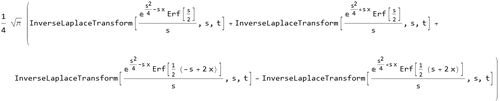
This is as far as Mathematica can go. Consulting tables of inverse Laplace transforms involving the error function didn’t help either. It is possible to use such tables to be able to write rules that transform Mathematica expressions. We could perform a numerical solution, but there is no point as it would reveal nothing in terms of the Laplace or inverse Laplace transform methods. A numerical solution works just as well for the original equation. This illustrates an important point, not every method is applicable or useful in solving every problem.
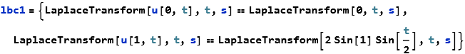
There are problems where this works. Let’s say we have a string of finite length, we can always scale this to a unit length. Say instead we have the Laplace transform.
![]()
We have the boundary conditions,
![]()
(11.9)
We then write.
![]()
We make these transformations.
![]()
![]()
We now solve the ODE.
![]()
![]()
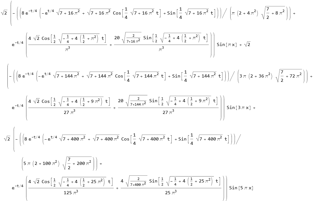
We transform this back
![]()
![]()
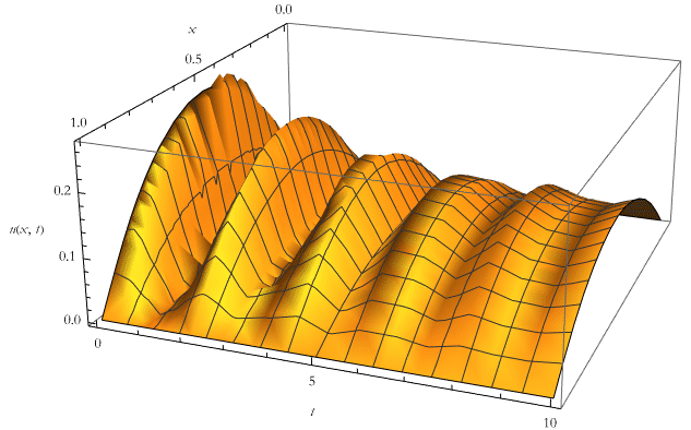
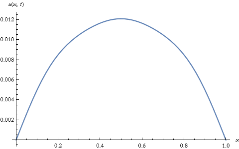
We can compare this to the DSolve result.
![]()
![]()
![]()
![]()
![]()
We get the same answer.
The Telegraph Equation
If we allow a damping effect γ, a restoring force coefficient β, and an external forcing effect f(x,t), then we can generalized the wave equation,
![]()
(11.10)
This is called the telegraph equation. Assuming c=1, β=1/2, γ=1/2, and f(x,t)=1, then we write this.
![]()
We write our quadratic initial conditions for our unit length string.
![]()
We fix the end points in the boundary conditions.
![]()
We construct the solution.
![]()
| |
|
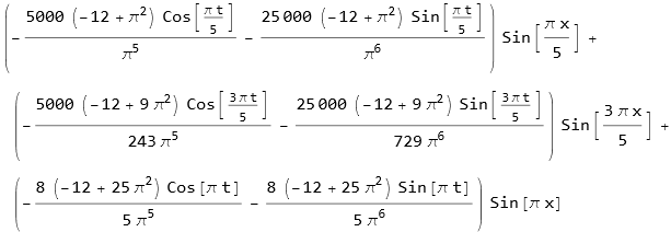
We extract the first five terms.
![]()
We can plot this.
![]()
![]()
Two Dimensions
As with the other classes of PDEs we have examined, we can extend this type to two spatial dimensions, too. For example, instead of a string, let’s say we have a rectangular membrane that is vibrating. Say this rectangle is a square such that 0<x<π and 0<y<π. In the absence of a damping force and where the boundaries are held fixed we can re write the wave equation,
![]()
(11.11)
and we can write the initial conditions,
![]()
(11.12)
where the boundary conditions are given as,

(11.13)
If the wave speed is 1, we can then write the equation and its IVBVP.
![]()
![]()
![]()
We can then build our solution.
![]()
![]()
We can find the first five terms.
![]()
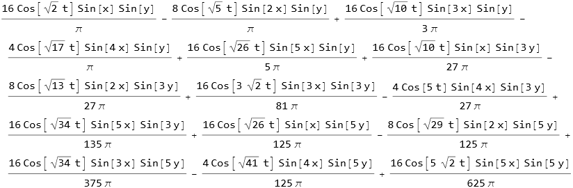
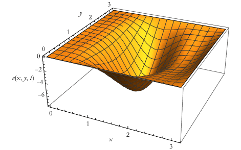
We can then plot this for a specific time.
![]()
We can animate this.
![]()
Three Dimensions
Of course, we can also extend the ability to solve PDEs to three dimensions. Here we study the vibrations of a parallelepiped of 3 units on a side. Again there is no damping. The IVBVP resulting is characterized by these equations,
![]()
(11.14)
![]()
(11.15)
![]()
(11.16)
![]()
(11.17)
![]()
(11.18)
![]()
(11.19)
![]()
(11.20)
![]()
(11.21)
![]()
(11.22)
We can write this system in Mathematica.
![]()
![]()
![]()
We then build the solution.
![]()
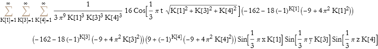
We can find the first five terms.
![]()
We can then plot this for a specific time.
![]()
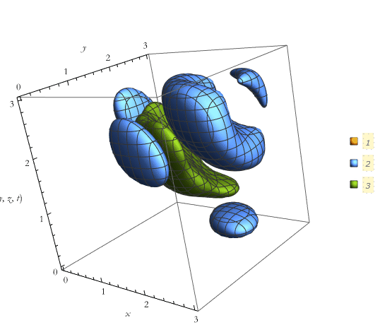
This plot took just over three hours to produce.