Parabolic Equations
George E. Hrabovsky
MAST
Introduction
In this lesson we look, in some detail, at the properties of parabolic equations. In specific we will study the heat and diffusion equations. We will explore many of the same issues we covered in the last lesson and then we will examine convection-type problems. We will examine systems with losses. We will also cover solutions over specific regions. We will end with a discussion of the time-dependent Schrödinger equation.
Heat Equation
Let’s say that we have a rod of length l. The temperature at any point along the rod is a function of the position along that rod, x, and time, t. Each material has its own ability to allow heat to flow through it, and this is represented by the symbol D (for diffusion, as we will see later). The equation that governs this flow of heat is called the heat equation, and is an iconic parabolic equation.
![]()
(10.1)
We can establish Dirichlet conditions at the end points, by assigning ![]() as the fixed temperature at x=0 and
as the fixed temperature at x=0 and ![]() for the fixed temperature at x=l.
for the fixed temperature at x=l.
![]()
(10.2)
For any real material the rod will start at some initial temperature, ![]() , giving us the initial condition
, giving us the initial condition
![]()
(10.3)
The nature of D varies depending upon the problem. For simple problems this is a parameter determined by the nature of the material. It might be a function of one or more variables. In some cases it is a tensor. While the heat equation in (10.1) might look fairly simple, the nature of D can make it arbitrarily complicated.
The Method of Separation of Variables
We can illustrate a method of solution called the separation of variables. If we combine the heat equation (10.1) with the boundary conditions of (10.2) and the initial conditions of (10.3) then we have what is called an Initial-Value Boundary-Value Problem (IVBVP). If we fix the temperature at the end points by the condition
![]()
(10.4)
The solution of this problem is then of the form
![]()
(10.5)
This solution is separable. If we substitute the solution into (10.1), we get,
![]()
(10.6)
Dividing through by D f(x) g(t), we get
![]()
(10.7)
These ratios are constant, we can assign the symbol λ to these, so
![]()
(10.8)
This in turn leads us to two ODEs,
![]()
(10.9)
and
![]()
(10.10)
The solutions for these are given below.
![]()
![]()
and
![]()
![]()
If we consider (10.4) we can write this f(0)=0=f(l).
![]()
![]()
So ![]() . We can then find the constant for x=l.
. We can then find the constant for x=l.
![]()
![]()
![]()
![]()
Naively, we can solve this to get the constant.
![]()
![]()
The problem with this is that we are seeking a nontrivial solution. So we need to look at exp2. This implies that
![]()
(10.11)
where n is some natural number greater than 0. We can substitute this into exp2 to get a general form for specific values of x.
![]()
![]()
Each of these values provides a solution to sol2.
We then have an infinite number of solutions based on (10.5), these solutions will be of the form
![]()
(10.12)
By the principle of superposition we can write
![]()
(10.13)
We can use this along with (10.3) to write
![]()
(10.14)
So,
![]()
(10.15)
are the eigenvalues for this problem. Similarly,
![]()
(10.16)
are the eigenfunctions.
Say that we have two eigenfunctions whose integer values are not equal, then we have the result.
![]()
![]()
So these eigenfunctions are orthogonal. If the two eigenfunctions share the same integer order, we get this result.
![]()
![]()
From this we can write an expression for the constants,
![]()
(10.17)
For any given eigenfunction we have this result.
![]()
![]()
We can insert this into (10.17).
![]()
(10.18)
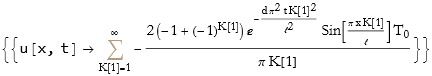
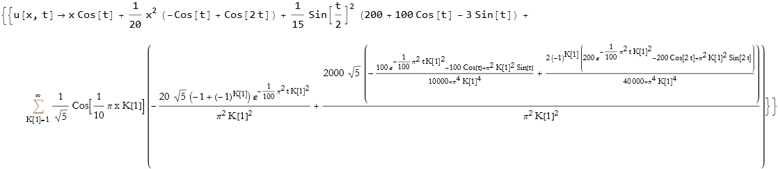
We can then substitute this into (10.13),
![]()
(10.19)
We can check to see if we get the same answer using DSolve.
![]()
![]()
![]()
![]()
![]()
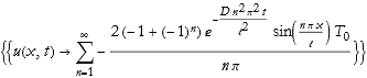
This takes a long time. The result is clearly the same as (10.19).
Dirichlet Problem
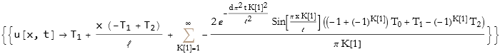
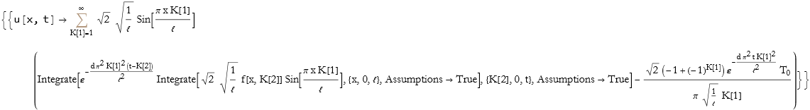
So what happens if the Dirichlet conditions are not 0? We write,
![]()
The solution for this is then given below.
![]()
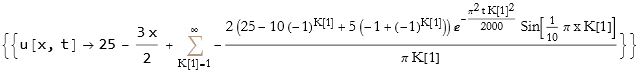
Now we need to specify some values. Say that the rod has a length of 10 units, the initial temperature of the rod is ![]() with the endpoint temperatures are
with the endpoint temperatures are ![]() and
and ![]() . Let’s also give a heat diffusion parameter of D=1/20. So we write it this way.
. Let’s also give a heat diffusion parameter of D=1/20. So we write it this way.
![]()
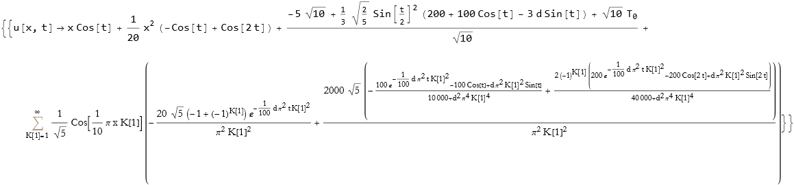
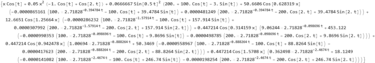
We can then extract the first five terms of the series.
![]()
![]()
We can plot this.
![]()
Steady State Problems
Over significant periods systems will achieve thermal equilibrium and the variation of temperature will fall away. So we can write,
![]()
(10.20)
for some function of position. We can also write,
![]()
(10.21)
We call this a steady state situation. The solution for this is then constructed.
![]()
![]()
We can rewrite this.
![]()
![]()
We can compare this to the limit of sol5 as t->∞,
![]()
![]()
![]()
Is this the same as exp10?
![]()
![]()
We can examine a plot of the previous situation for very long times.
![]()
Diffusion
The heat equation is a special application of the diffusion equation,
![]()
(10.22)
for some function of time and spatial coordinates, ρ, that represents density and where ![]() is a positive definite matrix of diffusion coefficients that may or may not depend on position and time—this is called the diffusion tensor.
is a positive definite matrix of diffusion coefficients that may or may not depend on position and time—this is called the diffusion tensor.
We write the diffusion equation.
![]()
![]()
We establish some initial conditions.
![]()
So can we solve this IVP?
![]()
![]()
This is a strange result, the density does not change through space and time. It is a bizarre prediction. Let’s try a numerical solution, given some specific value for ![]() . Also the diffusion coefficient will be treated as 1.
. Also the diffusion coefficient will be treated as 1.
![]()
![]()
![]()
![]()
The plot of this is given.
![]()
Let’s try another initial condition along with a continuous source term.
![]()
![]()
![]()
We can extract the first few terms of this series.
![]()
![]()
![]()

We can plot this.
![]()
We can compare this to the numerical solution.
![]()
![]()
![]()

So, what happens if this medium is in the form of a ring, we impose periodic boundary conditions.
![]()
We then get this solution.
![]()

We can extract the first few terms of this series.
![]()

![]()
We can plot this.
![]()
We can compare this to the numerical solution.
![]()
![]()
![]()
![]()
They are similar, but not the same. What happens if we take more terms in the series?
![]()
![]()
It has not changed, and it seems to almost violate the initial conditions along the x boundary, this is sensitive to the periodic boundary conditions. We can compare their difference.
![]()
The problem is due to the lack of compliance with the boundary conditions in the numerical solution, these issues fade away as the model continues to evolve in time. We can attempt to use the default method for NDSolve, the method of lines, but we will impose a pseudospectral method for the difference order due to the periodicity of the solution.
![]()
![]()
![]()
The plot of this is then give here.
![]()
Let’s see these two solutions plotted again st each other for t=0.
![]()

This points out the discrepancy between a series type solution and a numerical solution. Are we seeing an inconsistency in the conditions of a numerical solution? Or are we seeing artifacts due to Gibbs phenomena? No way to tell, here.
Neumann Problems
Returning to the heat equation, we can impose the Neumann conditions.
![]()
This gives us a new solution.
![]()
We can extract the first few terms of this series.
![]()
![]()
We can plot this.
![]()
Inhomogeneous Equations
In general we write the inhomogeneous heat equation,
![]()
(10.23)
We write this equation.
![]()
If we use the initial and boundary conditions defined earlier we can construct the solution.
![]()
Note that the solution is in terms of additional integrals. One way to cope with these is to rewrite them as numerical integrals. We can specify some values and resolve the equation. Let’s assume that f(x,t)=sin x.
![]()

We can extract the first few terms of this series.
![]()

![]()

We can plot this.
![]()
Convection
What happens if we have the same rod, but at the right end it experiences convective heat transfer. This convection is represented as a sink. We see this in the Robin-type boundary condition.
![]()
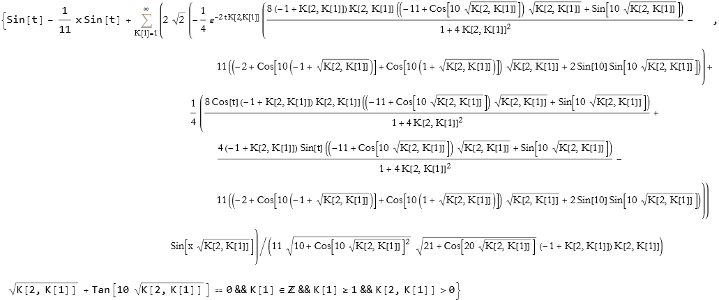
We can now write our solution.
![]()
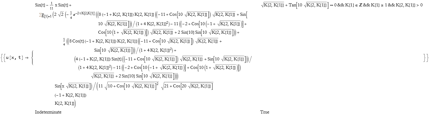
This is another example of the method of separation of variables. The infinite series is over the eigenfunctions that correspond to the eigenvalues listed as K[2,K[1]]. These eigenvalues are defined by the condition,
![]()
(10.24)
where K[2,K[1]]>0, K[1]≥1, and K[1]∈Z. If we want to plot our solution we need to calculate the eigenvalues that are within some range of values, say 0<K[2,K[1]]<500000.
![]()
How many eigenvalues are there in this range?
![]()
![]()
So we need to extract the first 1125 terms of the series corresponding to the eigenvalues.
![]()
We need to get rid of the conditional statements at the end.
![]()
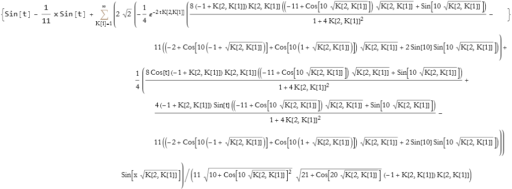
We now expand this by using the apply command @@.
![]()
We can then plot this.
![]()
Losses
How do we cope with the idea of a heat loss into the surrounding medium while fixing the temperature at both ends. If we represent this heat loss with the term η u, then we write,
![]()
(10.25)
So we write the equation.
![]()
We can write a set of boundary and initial values.
![]()
The solution is then given.
![]()
We can apply our values to this.
![]()
We can extract the first five terms of the series.
![]()
We can then plot this.
![]()
Unbounded Domains
What happens if our mythical rod is extremely long? We can treat it as semi-infinite. While the length may tend to infinity, we assume that temperature remains finite. We will continue to use eqn1 for this model. We will then write the initial and boundary values.
![]()
We can then write the solution.
![]()
![]()
Let’s fill in some values,
![]()
| |
|
We can then plot this.
![]()
![]()
Two-Dimensions
What happens if we want to extend our study to a rectangular plate instead of a rod? It is the same kind of equation,
![]()
(10.26)
To keep it simple let’s assume a square.
![]()
We can establish our initial conditions.
![]()
We have Dirichlet conditions for y=0 and y=10, with the temperature being zero there.
![]()
We assume the x=0 has a Neumann boundary that is insulated with a temperature of 0, and the other end has a Robin condition at x=10 and is in contact with a low temperature surrounding medium.
![]()
Instead of solving this symbolically and entering another rabbit hole of eigenvalues and eigenfunctions, I will solve this numerically.
![]()
![]()
![]()
We can plot this for any time.
![]()
We can make an animation.
![]()
Specific Regions
Here we define a region with a slit in it.
![]()
What does this look like?
![]()

We apply the same equation, eqn5. We will keep the initial condition.
![]()
![]()
We then construct a numerical solution.
![]()
![]()
![]()

So, we can rewrite our equation.
![]()
![]()
We test this for some specific time.
![]()
We can make an animation of this.
![]()
Time-Dependent Schrödinger Equation
We can write the Time-Dependent Schrödinger Equation (TDSE) in Mathematica.
![]()
We will apply Dirichlet conditions for two endpoints, a,b.
![]()
So, we can write the solution.
![]()
![]()
We can extract the first five terms.
![]()
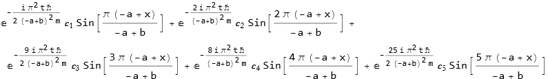
As an exercise, determine if this solution satisfies the equation given any set of constants.
So, let’s specify the initial conditions, a=0,b=1 and we will apply the natural units for h, and mass will also be 1.
![]()
![]()