Mathematical Operations for Computational Methods

George E. Hrabovsky

MAST

Introduction

We have come a long way from the days when we were forced to numerically solve problems if we wanted to use a computer. Modern systems are capable of symbolic and numerical computations at the same time. In this lesson we explore some of the fundamental concepts of operations to solve scientific problems by computer in the modern world.

The best model is based on a curve that we have perfect information about. People go to great lengths to assign curves to fit data. This leads to the belief that the curve so fitted corresponds to the behavior of the data and can predict the values of future data. Exact mathematical structures are the perfect basis of a perfect model.

So a model is an attempt to predict the future outcome of measurements. There are mathematical models that use the techniques of mathematics to make these predictions. There are computer models that use the techniques of computation to make such predictions. There are even physical models that are used.

The Marquis de Laplace once wrote, “We may regard the present state of the universe as the effect  of its past and the cause of its future. An intellect which at a certain moment would know all forces that set nature in motion, and all positions of all items of which nature is composed, if this intellect were also vast enough to submit these data to analysis, it would embrace in a single formula the movements of the greatest bodies of the universe and those of the tiniest atom; for such an intellect nothing would be uncertain and the future just like the past would be present before its eyes.”

This is the promise that modeling holds out to us. The problem arises that nature rarely, if ever, truly corresponds to exact mathematical structures. We thus need to approximate the structures in those cases where nature has chosen to be difficult. This leads us to numerical modeling.

The goal of a numerical model is to give an approximate, numerical, prediction of the behavior of a system.

Algorithms

In order to produce a numerical model we need to develop and implement a specific list of instructions that we call an algorithm. The word implementation here means that we have coded the algorithm into the computer language we choose for our problem solution. Of course, you can use an existing algorithm or implementation of an algorithm, but you should try hard to understand it. Executing algorithms is the heart of scientific computation. Here are some requirements for using algorithms in computational science:

Algorithms must not be ambiguous.

Algorithms must end in a definite way.

Algorithms must be complete.

The measure of how hard an algorithm is to execute is what we call the complexity of the algorithm. For example a system of n linear equations in n unknowns will require separate calculations. We call this a polynomial, or P, type problem. If the equations are actually nonlinear then there is no strict bound on the number of calculations required, and we call that a nonpolynomial. Problems that are polynomial can be performed in a specific time and with a specific amount of computer memory. A nonpolynomial type problem will generally take longer and require more memory than a P type problem.

For a polynomial type problem, we can get a quick and dirty measure of how complex a computation is by calculating the computational speed, s. If we know that there is some constant determined by the system that we will call k, and a constant that is determined by the complexity of the algorithm that we will call p, for some computational time t,

(1.1)

What is N? That is the number of computational points. What does that mean? Say we have a cube that we are modeling. If the length of a side of the cube is l, and we say that there are h number of points along each side, then the total number of points is

(1.2)

The distance between those points is the resolving power of the computation,

(1.3)

The Floating-Point Number System

I sit and look at my temperature sensor and it reads 86° F. I look at the news from yesterday and note the Dow Jones average was 35,120.08. The first number has two digits, the second has seven. We can look at the temperature number and look at it as likely accurate, but it lacks precision.  The Dow Jones average has seven digits and has more precision, but it almost certainly has needless information (why is a hundredth of a point significant?) There is a constant tension between accuracy and precision. As we know from mathematics representing real numbers that are not rational numbers requires infinite decimal expansions. These are impossible to calculate in their full detail. How do we solve this problem? We use a floating point number.

When we use a floating point number we must represent this on the computer. How do we do that? We apply something called a base-n floating point representation. Say that we have a floating-point number we want to represent, r, then

(1.4)

where s determines the sign of the representation, n is the base, f is the exponent, p is the precision, d is the digit, where p-1 is the least significant digit. In most microprocessors p is a fixed number. Each machine also has a maximum exponent that it can consider, if the absolute value of such an exponent exceeds that number the system returns a value of NaN (not a number). We often write (1.4) in terms of a positional notation,

(1.5)

There is a vast literature on the subject, here we can only scratch the surface. In some ways this is at the heart of the architecture for performing computational science.

Error

The problem with floating-point numbers is that they lose accuracy even as the precision grows. Every time you approximate a real number with a decimal expansion you are introducing error. Unless your calculations are entirely made up of exact results arrived at analytically there will be accumulating error with every subsequent computation. It is unavoidable. Eventually your computation will fill with error. If you do not know how fast this occurs then you will not know when your computation is no longer useful in predicting outcomes.

Here is a concrete example of what we were talking about with respect to floating point numbers. Say we have the simple quadratic equation

(1.6)

We can see by inspection that the two exact real solutions are given as

(1.7)

This leads to a common problem, the realization that on a computer we can never accurately calculate . We can approximate the solution, as we can see here.

The problem is illustrated if we go to a larger number of digits of precision.

When we approximate an irrational number error enters in. As we increase precision the error decreases (hopefully). Why not just go to twenty digits of precision? It adds to the computational cost of a calculation.

Here is another example, say we have a result that leads to the Taylor expansion of the cosine function

(1.8)

We can never calculate all of the terms required for this to be accurate. We have to stop somewhere, that introduces what we call a truncation error. For example, here we produce the Taylor expansion to fourth order,

Here we go to tenth order

Say we have a value of x of 3, the first result gives us

where the second gives us

As you can see the difference is startling. We compare it to the built-in function.

The first number is very far off.

By using Mathematica and its symbolic engine we can often avoid the problem that plagues purely numerical systems, like representing 1/10. In a purely numerical system we end up with something like this,

(1.9)

This is another infinite expansion and it has to be truncated at some point. Most systems will be off by about . We can check this.

The numerical estimate is,

Let’s look at a plot of the interesting function

(1.10)

That is a very nice curve. What happens if we look at a region very close to 0?

What the Hell is that?! If we look at (1.10) carefully we note that in the floating point representation 1 and cos 1 are almost the same and this results in a 0 result. This is called a cancellation error.

When using floating point numbers you should never check for equality. The fact that two floating point representations are the same does not imply that the numbers they represent are the same. Instead of checking whether two floating point numbers are equal you can do something involving some small tolerance, and we can call it ε. If the absolute value is within that tolerance we can think of two numbers as equal for all practical purposes. The finest tolerance available on a computer is the machine ε. You can find that with the $MachineEpsilon command.

So, in practical terms what is error? If we have a calculated result and an exact result, the absolute error is the difference between them.

(1.11)

More useful is the relative error,

(1.12)

Where do we get the machine ε? Say we have an approximate result that gives us a floating point number of having of +1 in the least significant digit. We can call this by the technical phrase, “One unit in the last place,” or with the equivalent symbol ulp. By applying (1.5) we get exactly the same absolute and relative errors, the result is the machine ε

(1.13)

Exercise: Determine your machine ε and figure out how to find the maximum allowable exponent p.

Limits and Differentiation

It is often required to represent a derivative in a computation. In numerical systems this is often accomplished through either computing the derivative and programming the resulting expression as a function or we use finite differences (see the next section). In symbolic systems we can compute these directly.

We can, of course, build the calculation of derivatives from first principles. For this we can use the Limit function in Mathematica. For example, if we have an expression of the form

(1.14)

and we want to find the limit as x->0, we can begin by opening a command line and typing [ESC] lim [ESC], then we use [CTRL] [SHIFT] (comma), then x right arrow (- >) 0.

The underscript used to be [CTRL] 4, but since version 12.2 they changed this WITHOUT TELLING ANYONE!!!!!

Using this method we can find the limit at a point, it can even be symbolic.

We can also examine what happens if x is allowed to grow without limit,

As an exercise examine the documentation for the Limit command and play with some examples.

We can use symbolic systems to calculate derivatives, too. We need not write,

then

We can use the D command

We can also use the ∂ operator

There is an extensive write-up of the D function, as an exercise go through it and make up some examples. Also look up the functions Derivative and Dt.

Finite Differences

Sometimes we will need to approximate a derivative. One way is the wrap the D expression in an N[].

Say, however, that we are interested in the derivative of an arbitrary function g(x) near the point x=0 on some evenly spaced lattice of points. If we get an expression for the derivative at x=0 we can always translate the solution to other values. We begin by writing the Taylor expansion of the function.

We can ignore higher orders by rewriting

We can see that the derivative of g is evaluated where x=0. We can see the effect of translating to adjacent points on the lattice (say x=±1),

we can do this for two point distances too,

We now make two equations,

and

We can see what happens when we subtract from

so our new equation is

We can solve this to get our approximation of the first derivative.

In most cases we can ignore the third derivative as it will become significantly small, though this will not always be the case. We can then rewrite this

This goes by a special name, it is a 3-point formula.

If we want to use this in a Mathematica program we would write function of this kind,

For example, if we use this for the sine function.

We can test this

The error is given by (1.11)

That is a reasonable result.

Exercise: Use the method described above to generate a 5-point formula.

Exercise: Develop a formula to calculate the second derivative.

We get the same result using the built-in DifferenceQuotient function.

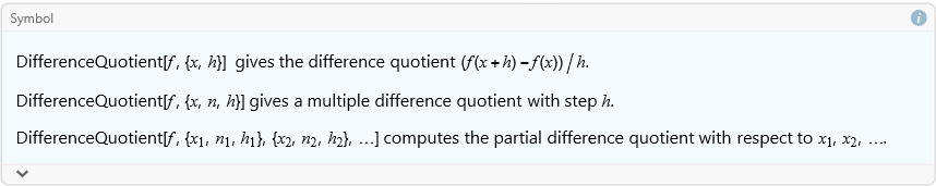
Here we write the symmetric difference quotient.

Integration and Quadrature

Mathematica is capable of calculating antiderivatives using the Integrate[] command. For example,

Of course, this is an antiderivative and not really an indefinite integral. To accomplish an actual integral we insert a subcommand within the integrate command called , GeneratedParameters.

We can calculate a definite integral.

As an exercise look through the extensive write-up on the Integrate function and work some examples.

It is often necessary to introduce a numerical approximation of an integral. Compare this with the definite integral.

There are many options for making this accurate and precise. You should explore the options that are available. One aspect that requires additional attention is the option Methods. To find the listing of the available strategies and rules find the Advanced Numerical Integration tutorial. This online document contains the details of the various methods you can use. Go through this document when you want to use a specific method.

To be clear, Mathematica can choose automatically the method being used if we do not specify a method. We can choose the method as we like. Let’s try a somewhat more challenging integrand,

At zero we have a problem.

Close to 0 we are doing fine.

Assuming that the integral can exist, we proceed. We will examine two different integrations, one including the indeterminate limit and the other nearby. This will help us to test the capability of the integration method. If the two are close, then we can have some confidence.

This is pretty good. Let’s look at some different methods,

it is clear that the Trapezoidal rule does not cope well with the rapid oscillation of the integrand.

We can see that the standard Newton-Cotes rule does not apply either. What about Gaussian quadrature?

We can extend this with the Kronrod rule.

By this point we should expect any polynomial-based method to fail. Here we try the Levin rule.

This worked pretty well. Here we sample some strategies.

This one worked.

This one did not.

As an exercise, play around with the different methods and strategies.

Interpolation

Interpolation is the creation of a function that connects a set of points. To accomplish this we get something called an IntrpolatingFunction that we can use just like any other function. In Mathematica we use the FunctionInterpolation[] command to interpolate a function statement.

What we have done is use the system to generate points and then interpolate them. We will explore the interpolation of data points in the next lesson. As I said, we can use this just like any other function. For example, here we plot the interpolating function along with its first and second derivatives.

We will explore specific interpolation methods throughout the course.

Root Finding

What does it mean to find the roots of a function in one variable? Given an arbitrary function f(x), the roots are the set of N variables , such that,

(1.15)

Given a function we can determine the roots of that function using the FindRoot[] command. The requirement is that we choose some starting point for the recursion to start at, . Here we can find the roots of a simple polynomial.

As with many Mathematica functions, there are a list of methods that you can use in FindRoot[]. Unfortunately, also common in Mathematica, there is no published list of these methods. I will try to list many of the methods here. Here we introduce a function that has well-defined roots.

We can see the behavior of this function in a plot.

We can see that the first root should be around π, and subsequent roots are multiples of π.

The method found the first root just fine, but later ones are not done well. The default uses Newton’s method, and it is clear that in this case it does not do well.

The secant method found no roots.

We can make a table for this.

This did well. Let’s see what happens if we list a method not within the system.

This tells us that the known methods are Brent, Secant, AffineCovariantNewton, and Newton. The Brent method is only applicable if we can bracket the root.

This also did well.