Computational Interlude #1: Introduction to Mathematica
A Note to the Reader
If you do not have access to Mathematica, or you do not want to get it, you can ignore this lesson. You can always come back to it later.
Introduction
This lesson will introduce Mathematica (MMA) and its underlying programming engine the Wolfram Language (WL) from the perspective of a new user. We begin by discussing why MMA is revolutionary and why you should use it. We will also discuss some myths that have grown up around MMA and WL. We will examine the origin and evolution of MMA from its beginnings to the present day. We will then discuss the structure of MMA and why it is important to understand it. We will then turn to a lengthy presentation of how to use MMA for performing calculations. We then turn to the issue of using MMA for visualization of function behavior. We then have a discussion of how to get more information within MMA. We will end with details of lists, matrices, and vectors.
Computers are electronic devices that are capable of acquiring, storing, and manipulating data in the form of binary codes. The first electronic computer of this type was made in the mid to late 1940s to assist in calculations required for the development of the hydrogen bomb. Since then, computers have become an integral part of daily life. With modern computers you can collect data from instruments and experiments and store it in files, you can analyze the data, you can construct predictive models, display the data and the predictions, you can write up the results and present them in web pages, journals, and live presentations.
Broadly speaking, a computer consists of a central processing unit (CPU) that controls everything, a memory unit that stores information for active use by the CPU, peripheral devices for display, long-term storage, printing, and communication with other computers, and the computer also has one or more buses for connecting all of the elements of the computer together. We communicate with a computer through a keyboard and a display monitor, and we often use a mouse or a track ball.
In order to make a model that operates on a computer you must be able to write out a complete list of instructions telling the computer what to do. Such a list of instructions is called an algorithm. Computers all have a language that is unique to their CPU called a machine language. Few people communicate directly with the computer in machine language. Most algorithms can be converted to machine language from some other programming language through some kind of interface. Such interfaces use either active conversion as you write each instruction (this kind of language interface is called an interpreter), or the algorithm is written in its entirety and then converted all at once to machine language (this is called a compiler). The process of translating an algorithm into a computer language is called coding. A translated algorithm is called a computer code or program. Often a computer language will have a special program that contains a place where code is written, other places where information about the language is stored for reference, and there can even be tools to assist in writing your code; such a program is called a programming environment.
To operate, or run, a program the first instruction of the program is directed from long-term storage to the CPU and it acts on any relevant data that is kept in long-term storage for this purpose. Once this is completed the results are placed in memory. The CPU is then directed to the next instruction and the process is repeated. This continues until every instruction has been completed.
Mathematica is a programming environment that uses the Wolfram Language as its computer language. The place where coding takes place is most often in a place called a notebook. The notebook is often an interpreter, though WL has a compiler that is becoming integrated into more and more functions with every new version release and it allows you to compile complicated instructions so that they run faster. Thus MMA can be thought of as a hybrid interpreter/compiler.
There are hundreds of computer languages and dozens of programming environments—many of them are free. This being the case, why choose Mathematica? MMA has many useful aspects that are not individually unique to it, but are collectively unique. MMA/WL is platform independent (it does not depend on which operating system or CPU you use). It allows you to create programs based on algorithmic procedures (called procedural programming and this style of programming is familiar to everyone who has programmed in C, C++, Java, Python, etc.), WL also allows you to manipulate combinations of instructions (what we call functional programming), it allows you to rewrite instructions by applying rules (what we could call rule-based or transformational programming), and you can mix and match these kinds of programming as you like, you can create reports and finished papers (this lesson is written entirely in Mathematica, for example), you can import and export data, you can perform calculations that are entirely symbolic, you can perform calculations that are entirely numerical, and you can perform calculations that are both symbolic and numerical. There is no other system that has all of these capabilities that are free.
The professional/academic version of Mathematica is available from Wolfram Research and it allows you to produce code and sell it, to write technical documents (such as this lesson) and sell them, or to provide consulting services for pay. There is a version that is entirely in a cloud that you can log into over the Internet. There is a reduced price version for hobbyists, the caveat is that you cannot use this version for making money. There is also a version for use by students with a valid student ID. All of these versions of Mathematica are the same in terms of functionality.
There are some oft-repeated statements made about MMA/WL that are not true. Many people choose not to use MMA because it is slow compared to some other language. It might be true that optimized code in a special language might be a few percent faster than MMA, but there are two things that need to be pointed out. If you convert directly from, say, a procedural language to procedural code in MMA it is not the most efficient use of MMA. It is better to choose what parts of MMA are best for the algorithm you want to code (perhaps even changing the algorithm). The other thing to consider is development time, MMA requires only a fraction of the time to code as other languages. If you optimize the implementation of an algorithm in MMA/WL it will run competitively.
Another complaint is that MMA is a black box, where you have no idea what is going on once you start using a built-in function. It is true that some functions in WL or MMA are so complicated and huge that the specific method being used is not easy to follow. There is a continual struggle to document functions and methods that often lags behind development. On the other hand you are not restricted to use built-in functions. If you are uncertain about how something is being done, write your own code. Compare it with the built-in function.
Another complaint is that MMA/WL can only handle small projects on a desktop computer. That is sheer nonsense. Wolfram|Alpha is an online interactive system maintained on a large cluster of computers accessible to anyone over the Internet and consists of millions of lines of MMA/WL code alongside C++ code.
What is a Computer Algebra System (CAS)?
This is a now, mostly, outdated term to describe systems that allow you to perform symbolic mathematical operations on a computer instead of the tradition numerical operations. I consider it outdated because neither of the two principle systems (Mathematica and Maple) are strictly algebra systems, as they both have very robust numerical and general programming capabilities.
The first CAS I know of was called MathLab and came out in 1964. It brought about what can be considered the first generation of CAS. These are exclusively written in, and require the use of, the programming language LISP. Reduce came out in 1968, it is now in the public domain. Reduce is also a first-generation system—it is written in, and requires, LISP. It is freely available from the website: http://www.reduce-algebra.com/ . Then Macsyma was developed in 1969. This had an interesting development path. Macsyma was sold commercially for a while, and is now defunct. MIT had a version of it under the DOE, called Maxima, which entered the public domain. This is now available at the website: http://maxima.sourceforge.net/ . Scratchpad was the next first-generation system and it came out in 1974. This is was a remarkable system that later became Axiom. Axiom is now terribly out of date, at least in terms of its interface, and is available at the web site: http://axiom.axiom-developer.org/ . MuMath, which later became Derive, came into being in 1979, and was the last of the first-generation systems developed in LISP. Derive had an interesting life. Starting out as a reduced-strength CAS for students, it saw life in certain powerful hand-held calculators.
SMP (Symbolic Manipulation Program) was pretty revolutionary for its time, it was developed by Chris Cole and Stephen Wolfram in 1981 while they were at Caltech. Maple is a second-generation system written in C and C++ and first arrived in 1983 from Waterloo Software (now owned by Cybernet Systems Group). It is now a fully capable environment for programming and scientific discovery.
Mathematica came out in 1988, also written in C/C++. Depending on who you talk to, it is the most popular of the general CAS. When Stephen Wolfram left Caltech he was unable to take SMP with him, as it was being sold by a different company. Wolfram, along with other developers produced the first commercial version of MMA in 1988 where it had approximately 500 functions. Each new version added new functions where the newest version has more than 6000 built-in functions. Of course, it has always had a programming language that in 2013 was officially named the Wolfram Language (WL). So, if it doesn’t do something you want it to do, you can program a new function or even a large software system.
MuPAD came out in 1992 and is available only as a MATLAB add-on. I consider this to be extremely expensive, since you need MATLAB and then MuPAD.
The Structure of Mathematica
When you start Mathematica it loads into memory from long-term storage. The link to the CPU is called the Mathematica Kernel. It also loads a user interface file called the Notebook Front End, or just the notebook. Multiple notebooks can be loaded at once. Notebooks can be saved into long-term storage once you name them. You can load special programs that extend the capabilities of the kernel, these are called packages.
Most of the work done in Mathematica takes place in the notebook. This front end interface easily allows you to write programs, include text, graphics, and even sound into one place. An important aspect of notebooks are the brackets that appear on the far right side, these are called cells. All instructions appear in cells. A cell encompasses a paragraph. They are the basic element of a notebook. You can copy and paste cells, you can change their format, and you can execute any instructions contained in such a cell. In Windows you place the cursor anywhere in the instruction you want to execute, or you highlight the cell (by clicking on it), and then you hold down the Shift key and press Enter.
If you have a multiprocessor computer, then you can have a number of kernels running in parallel, one on each of a number of processors (usually half the number of processors you have on your computer). If you have a network of computers, and each computer has MMA, then you can connect them over a local-area network (LAN) by using the built-in Lightweight Grid. This allows you to have different processes operating on multiple cores or multiple computers.
The fundamental object that is placed in active memory is called an expression. Everything you work on in a cell is an expression, whether it is a calculation, a paragraph of text, an image, a sound file, a video, or any combination. MMA/WL has a sophisticated system for interpreting expressions. Say we have the expression a+b. This is an expression made up of three sub-objects that we can call tokens. There are two symbolic tokens, a and b, and one operator token +. MMA/WL looks at the expression and sees the operator first in the form of a header, Plus, then the symbols, so it sees Plus[a,b]. Simple expressions can be used to build more complicated expressions.
New functions can be created in notebooks. Sometimes, especially with large collections of functions we might place them all into a special notebook that we call a package. A package is stored in a folder called AddOns and as you might expect they are loaded to add new functionality to MMA/WL.
Using Mathematica for Calculation
Arithmetic
Mathematica allows you to perform each arithmetic operation and its inverse. To add two numbers, say 454 and 63, we open an Input Cell and write
![]()
![]()
Exercise 3.1: Add any two numbers using Mathematica. Type list1, then =, this will immediately assign whatever follows to the name list1. You can make a list by writing a curly bracket, {, and then listing each number with a comma separating each, and then closing the list with the end curly bracket, }. Execute this command, placing list1 into active memory. Type ?Total to get the write-up of the command Total. In a new line write Total[list1] in order to get the sum of all the elements of your list.
To multiply two numbers, say 64 and 5155158, we can write
![]()
![]()
or we just put a space between the factors,
![]()
![]()
Note that MMA fills in a multiplication symbol when applying the space to numbers.
Exercise 3.2: Multiply any two numbers.
We can raise a number, say, 55 to a power, say 8,
![]()
![]()
we can also type 55 and then the command Ctrl 6 and then 8.
![]()
![]()
Exercise 3.3: Raise any number to some power.
We can take the inverse of addition, subtraction by writing
![]()
![]()
Exercise 3.4: Subtract any number by some number.
The inverse of multiplication is, of course, division,
![]()
![]()
Exercise 3.5: Divide any number by some number.
The first inverse of raising a number to a power is to take the power-order root (the surd) of the exponent to get the base. Here we use the command Surd, followed by square brackets [], the square bracket is standard notation for the arguments of a built-in function.
![]()
![]()
we can also write this using a fractional power.
![]()
![]()
Exercise 3.6: Find the Surd of any number to some fractional power.
The second inverse of raising a number to a power is to take the base logarithm of the exponent to get the power, here the base is 55.
![]()
![]()
Exercise 3.7: Find the logarithm of any number to some number base.
Let’s say we wanted to find the 9th root of our exponent,
![]()
![]()
this is an exact result, and it is very difficult to interpret it. It would be better if we could get a numerical approximation of this, we can take the previous expression and wrap an N[] around it to get a floating-point approximation.
![]()
![]()
Or we can write //N after the expression.
![]()
![]()
Or we can specify that we want the surd out to as many as ten decimal places
![]()
![]()
of course it doesn’t give more digits than are needed.
Exercise 3.8: For previous answers that were difficult to interpret, find the numerical approximation to some number of digits of precision.
Symbolic Calculations
As stated above, we are not restricted to numerical calculations. When doing symbolic calculations it is a good idea to assign a name to each expression as you enter it. We will use the immediate assignment symbol = to assign an expression to our label. Here we invent three expressions
![]()
where the semi-colon symbol ; tells Mathematica not to display output.
Exercise 3.9: Create an algebraic expression and assign it the label of ex1.
We can take a power
![]()
![]()
Exercise 3.10: Raise your created expression to some power, label this ex2.
we can expand this expression.
![]()
![]()
We can take the product.
![]()
![]()
Exercise 3.11: Expand ex2 and name this ex3.
We can simplify this.
![]()
![]()
We can take the quotient
![]()
![]()
and we can factor this
![]()
![]()
We can write an equation in Mathematica by using the logical equals symbol ==. The single = tells Mathematica that we are assigning an expression to a label, the logical equality == tells us that we have an equation.
![]()
Exercise 3.12: Create an algebraic equation and label it eqn1.
We can solve this for t.
![]()
![]()
We can specify the first solution using the symbol for the element of a list,
![]()
![]()
or the second
![]()
![]()
Exercise 3.13: Solve eqn1 and label the solution soln1.
Physical Quantities
If we want to specify that a physical quantity is being considered, where we have a numerical coefficient of a physical unit, we can do this in Mathematica by using the Quantity command, Quantity[magnitude,unit], here the magnitude is the coefficient and unit is the unit of measurement being used. For a distance of 10 m we can write,
![]()
![]()
you can use this format to encode any physical quantities.
Mathematica knows all of the measurement systems in use, all you have to do is specify the unit and it knows how to display it.
Let’s assume that you want to show a ratio between distance and the time it takes to cover that distance. We start with d1 above and say it took 10 seconds to cover it,
![]()
![]()
We can convert this to feet in the English system,
![]()
and we can get this as a decimal approximation, and if you place the cursor over the result it reveals the units.
![]()
![]()
or even to Light Years (the distance light travels in a Year)
![]()
![]()
Algebraic Operations
There are two powerful commands for simplifying expressions. The act of simplification is a set of transformations that result in the most reduced form of the expression. The first is Simplify[expression]. Here we have a simplification of a polynomial.
![]()
![]()
Note that the order is reversed from the way most of us would write it. We can use the // to put a command at the end of the instruction. We can use the instruction TraditionalForm to write the answer in a nice font and in a way that matches how we might write on a note pad.
![]()
![]()
Here we have a rational expression.
![]()
![]()
Sometimes we will need to make assumptions clear before getting the answer we want. Here is an example.
![]()
![]()
While this is true, it is not very useful. We note our assumption that x∈R,
![]()
![]()
That’s better.
We can also use the Assuming command first,
![]()
![]()
FullSimplify can be used if Simplify is not effective. Warning FullSimplify takes more time.
![]()
![]()
Expand allows you to expand products and integer powers. For example.
![]()
![]()
![]()
![]()
PowerExpand allows you to expand all products of powers and roots.
![]()
![]()
![]()
![]()
We can use ExpandAll when we have a combination of sums and powers.
![]()
![]()
Factor allows us to factor a polynomial.

![]()
Collect[expression,form] collects terms of powers that match the form specified.
![]()
![]()
We can simplify this,
![]()
![]()
Together places the terms into a sum over a common denominator

Refine allows us to convert a symbolic expression to one where a numerical factor would be included, returning to an example from above we see
![]()
![]()
![]()
![]()
Distribute allows us to apply the distributive law over an operator, in this case multiplication,
![]()
![]()
Distribute does not perform the addition in the correct order, so the product disappears.
![]()
![]()
To do it correctly we can use the command Unevaluated around the product, this allows the product to be done in the correct order.
![]()
![]()
Apart makes a rational expression into a sum of minimal denominators,
![]()
![]()
Trigonometry
Here are some examples of trigonometric expressions, these apply relevant trigonometric identities.
![]()
![]()
Simplify does this automatically.
![]()
![]()
PowerExpand does not,
![]()
![]()
instead we use TrigExpand
![]()
![]()
TrigReduce should reverse the expansion.
![]()
![]()
Why did it fail? TraditionalForm is the problem. How do we get expressions to work correctly and display the way we want them to? Wrap the TraditionalForm around the expression instead of applying it at the end.
![]()
![]()
![]()
this does not change the expression,
![]()
![]()
![]()
![]()
Equation Solving
Mathematica can symbolically solve equations, note that the result is in the form of a transformation.
![]()
![]()
We can remove a level of brackets by specifying the first solution.
![]()
![]()
Or we can tell Mathematica to display the solution and transform the symbol for x according to the solved equation.
![]()
![]()
We can reproduce the quadratic formula. There are two solutions, so the result is a list of two solutions. We can specify the first element of the list.
![]()
![]()
Here is the second element of the list of solutions.
![]()
![]()
Mathematica can solve systems of equations, too.
![]()
![]()
![]()
![]()
![]()
![]()
Or we can perform a real approximation of these exact results,
![]()
![]()
Using Mathematica for Visualization
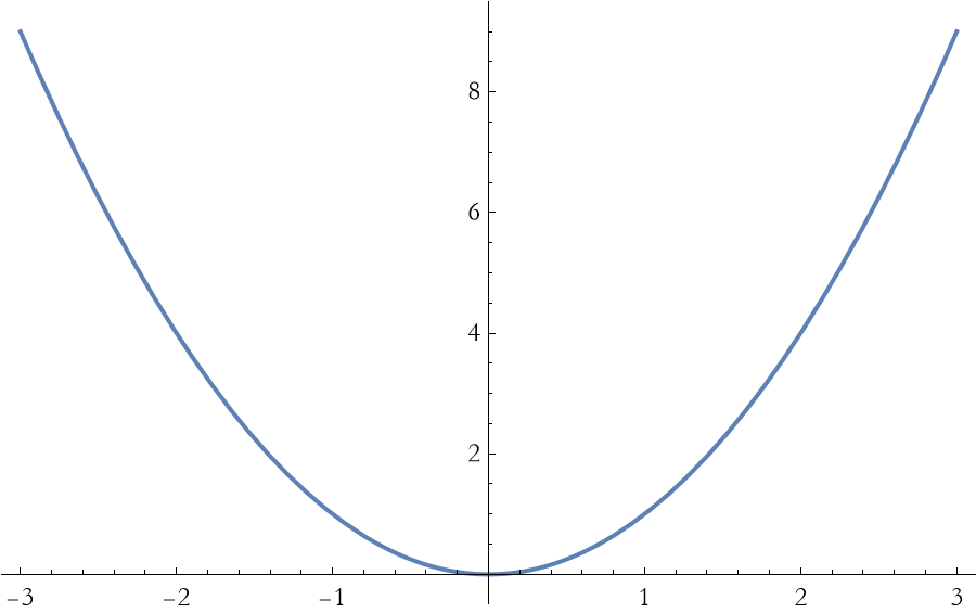
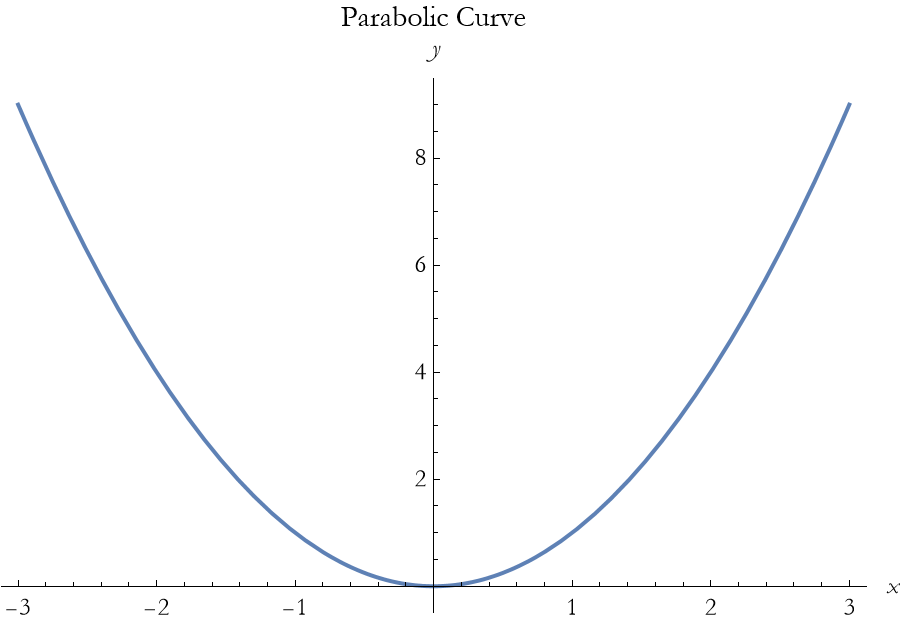
The plot command plots an expression for an independent variable over a specified range of values.
![]()
We can easily make this plot useful to all viewers by labeling the axes with nicely formatted labels, and providing a label for the plot itself. Show allows us to combine many graphics command into a single unit. GrayLevel->0 is the value for black.

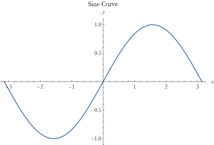
Here we show how Mathematica handles a trigonometric function.
![]()
Using Mathematica as a Scratch Pad
One of the uses of a Mathematica notebook is the way that you would use a page of a scratch pad. You write down the expressions you want to use, you specify the physical quantities involved, and then you can perform your calculations.
Most of you have done this with a sheet of paper, where you start by writing out what you know and then working the problem through successive calculations, notes, and diagrams.
You can easily use MMA notebooks as scratch pads in the same way.
Using the Mathematica Help System
You can look things up in the documentation systems. If you note the Help Menu at the top of the notebook, you can access the system there. When you choose the Help Menu you then choose Wolfram Documentation and a user interface window opens up.
If you know what you are looking for you can type it into the search bar at the top of the screen.
You might not know what you are looking for. There are four main parts of the interface to find what you want. First, there are a series of colored blocks that you can click on. Then there are a number of gray buttons entitled workflows. Another set of gray buttons called resources. Finally there are four text-based links at the bottom.
Examining the colored blocks you will note four colors. The orange blocks are six aspects of the system itself. The yellow blocks represent types of expressions. The green blocks represent types of applications. The blue blocks represent deliverables.
The six orange blocks are Core Language and Structure, dealing with fundamental aspects of the Wolfram Language and how to program in it. Data Manipulation and Analysis are a collection of aspects relating to collections of data that you as the user provide. Visualization and Graphics explore how to represent functions and data. Machine Learning is where you can look up functions allowing you to construct machine learning capabilities, that is to teach the machine to do a number of tasks in an almost autonomous way. Symbolic and Numeric Computation covers using WL to perform mathematical operations. Higher Mathematical Computation deals with advanced mathematics.
The six yellow blocks begins with Strings and Text, these are functions that allow you to process strings and text in programming. Graphs and Networks allow you to explore such objects a directed graphs and the subject of both graph theory and its related network theory. Images explores the MMA/WL ability to analyze and enhance images. Geometry explores geometrical objects. Sound and Video allow you to analyze and enhance audio files and video files. Knowledge Representation and Natural Language explore how MMA/WL uses knowledge-type structures in programming.
The six green application blocks begin with Time-Related Computation, exploring time-based dynamical systems. The remaining green blocks have collections of functions allowing you to explore curated data and applications of a specific nature: Geographic, Scientific and Medical, Engineering, Financial, and Social/Cultural/Linguistic.
The six blue deliverable blocks begin with Notebook Documents and Presentation that collect functions allowing you to control various aspects of notebooks that you can program to create documents, web pages, reports, and slide shows. User Interface Construction explore functions allowing you to create graphic user interfaces (GUIs) for any occasion. System Operation and Setup are functions that allow you to tailor your use of MMA/WL. External Interface and Connections are functions related to networking and how to share information. Cloud and Deployment are functions related to cloud-type environments. Recent Features explore new functions from the most recent versions.
There are twelve workflow blocks. What is a workflow? A workflow is a repeatable pattern of activity to provide some service or to process some kind of information. You can think of it as an algorithm connecting materials, services, and information through a sequence of operations. In MMA/WL the workflow buttons provide suggestions on how to proceed with specific types of workflows.
The six Resource blocks provide resources to support your continuing development as a MMA/WL user/programmer. One homework assignment will be to work through one, or both, of the fast introductions. The Intro Book and Course connects you via the Internet to an online version of Stephen Wolfram’s introductory book in programming in the WL. Archives and repositories connect you to one of several online collections maintained by Wolfram Research. The function repository is very useful as it contains user-developed functions not implemented into MMA/WL but are useful (in fact you can create your own functions and share them here for other users). Resources for Software Developers are a collection of free tools for developing software (including free Wolfram Engine for developers), there are also other development environments that you can download. There are other Wolfram Language products than MMA. Then there are a number of educational resources through Wolfram U.
Palettes are arrays of buttons that produce specific output can be found in the Palettes menu. Many of these are useful and you can, or course, create your own.
If you are in a notebook and you want to find out about a function you are using, you can type a question mark and then the function name. For example,
![]()
I will end with a warning. The documentation in MMA consists of literally thousands of pages of free resources. It is very easy to get sucked in while searching and spend hours poking around. It is usually fun and you almost always find new things. Beware of getting sucked down these rabbit holes, it happens to me all the time!
Lists, Matrices, and Vectors
It is rare when you have only a single value for a variable. Mathematica allows you to manipulate lists of expressions. You can create them manually using curly brackets.
![]()
![]()
We can also use Range[ ]
![]()
![]()
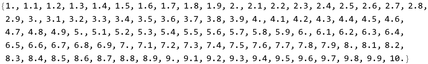
We can increase the number of values in a Range by including a statement of how many intervals we have between the numbers specified. Here we have the same range, but we have a new value every tenth of a number.
![]()
You can create lists using a table, Table[ ]
![]()

We can see this as an actual table using the TableForm command.
![]()
| 1 | 1 | 1 |
| 2 | 4 | |
| 3 | 9 | |
| 4 | 16 | 2 |
| 5 | 25 | |
| 6 | 36 | |
| 7 | 49 | |
| 8 | 64 | |
| 9 | 81 | 3 |
| 10 | 100 |
We can extract elements of a list or a table. For example, to extract the 13th element of r2 is given by naming the list and the list element label in double square brackets [[13]],
![]()
![]()
What happens if we look at the 3rd element of a table, like valtab?
![]()
![]()
What is we want the second element of this list?
![]()
![]()
How do we enter a matrix into Mathematica? The simplest way is to go to the Insert menu above. Choose Table/Matrix. Then choose New. Click Matrix. Then specify the number of rows and columns. I chose 2 each. Then click on OK. This is what you get.
![]()
You can enter what you like into the spaces.
The limitation of this method becomes apparent in two cases. The first is if the matrix is large. The second is if the matrix has definite values based on some method or process.
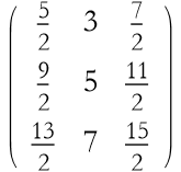
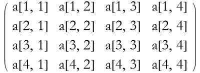
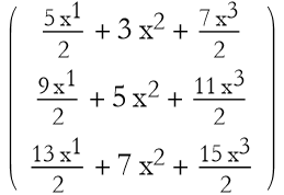
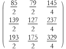
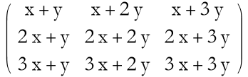
For these situations we use the Table[] command. For example, if we have a 3×3 matrix whose elements are given by a formula, then we might write what follows.
![]()
![]()
We can see this in matrix form.
![]()
We can also use the Array command.
![]()
We can construct an array of the coefficients of a list of polynomials using the CoefficientArrays command.
![]()
![]()

![]()
![]()
![]()
![]()
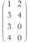
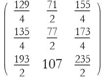
We can combine two matrices by using the Join command.
![]()
![]()
We can use all of the list commands to pull out the elements of a matrix. Here we take the third row of our first matrix.
![]()
![]()
Here is the second column.
![]()
![]()
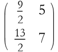
We can also get a submatrix using the Take command.
![]()
![]()
We can also take pieces away from a matrix to make a new matrix by using the Drop command.
![]()
Here we remove the first row from exp1.
![]()
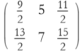
Here we remove the first column.
![]()
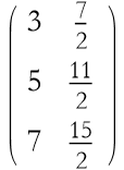
If we want only particular parts of a matrix we use the Extract command.
![]()
Here we extract the first row from exp1.
![]()
![]()
Here we extract the first column.
![]()
![]()
Given a full array, one whose rows and columns form a rectangular array, we can get a list of the dimensions of the array using the Dimensions command.
![]()
![]()
![]()
![]()
![]()
![]()
An array that is not full is sometimes termed ragged.
![]()
![]()
In this last case the first row determines the size of the array, the other rows do not have the same number of elements, so we call this ragged.
We can extract the diagonal of a matrix using the Diagonal command.
![]()
![]()
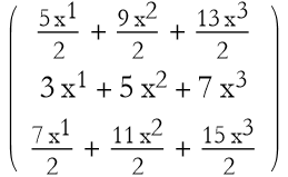
We can transpose a matrix.
![]()
Transpose can also be accomplished by typing [ESC]tr[ESC]
![]()

As an exercise read through the documentation on Transpose and work several examples.
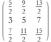
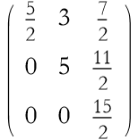
If we want to keep all of the upper triangular elements as they are, but all other elements become zeros we use the command UpperTriangularize.
![]()
![]()
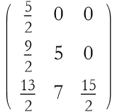
We can do a similar thing with the LowerTriangularize command.
![]()
![]()
It is also possible to change an element of a matrix using the ReplacePart command.
![]()
For example, we can change exp14 to have a 4 in the {1,3} position.
![]()
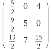
Determinants are also easily found.
![]()
![]()
Symbolically
![]()
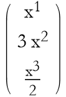
From the perspective of lists and matrices, a vector can be represented as a one-dimensional matrix, either a column or a row. In fact, the default representation of a vector is written as a row, but it is treated as a column vector. Any method that allows you to make a matrix can, therefore, be used to construct a vector.
![]()
![]()
This seems to be a row matrix, but if we apply MatrixForm we see that it is a column matrix.
![]()
![]()
A row matrix is constructed this way.
![]()
![]()
![]()
![]()
We can multiply a vector by a matrix.
![]()
We can see that the order of multiplication is important.
![]()
We can also multiply matrices,
![]()
Again we see that the order of multiplication is important.
![]()
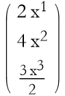
Let’s say that we define another vector.
![]()
We can add vectors.
![]()
Scalar multiplication is accomplished in a completely intuitive way.
![]()
The scalar product is accomplished using the . symbol.
![]()
![]()
You can also use the Dot command.
![]()
![]()
We can find the norm of a vector using the Norm command.
![]()
![]()
Say we have another vector.
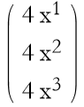
![]()
![]()
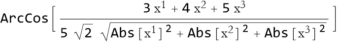
We can find the angle between vectors by using the VectorAngle command.
![]()
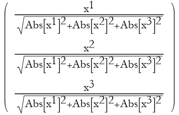
We can use Normalize[] to find the unit vector in the direction of vec1.
![]()
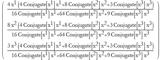
How do we project vec1 onto vec2?
![]()
As an exercise look up the documentation on Normalize, Projection, and Orthogonalize and work several examples of each.
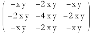
We can plot a matrix.
![]()
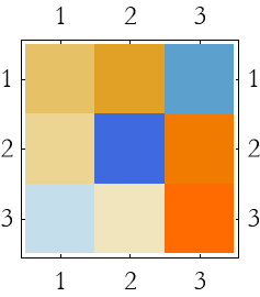
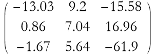
We can invert a matrix and see a plot of it.
![]()
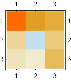
As an exercise read through the documentation on Inverse and MatrixPlot (and also ArrayPlot), and work several examples.
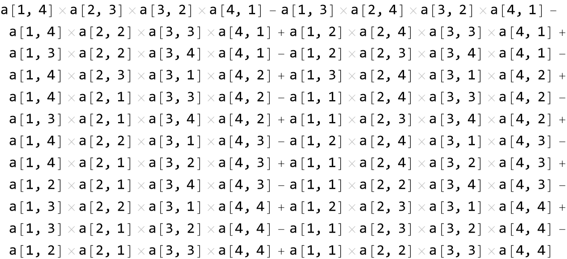
Here is a program from the Wolfram documentation on how to calculate the cofactor of a square matrix.
![]()
We use this to find the cofactor of mat16 removing the 3rd row and second column.
![]()
![]()
As an exercise read through the documentation of Det and work several examples.
We can also find the minors of a matrix.
![]()
We can also use this on symbolic matrices.
![]()
Here we compare it to the original matrix.
![]()
As an exercise read the documentation for Minors and work several examples.
We can find the trace of a matrix.
![]()
![]()
As an exercise read the documentation for Tr, note particularly the program for calculating the inner product of a cone of positive definite matrices. Work several examples of your own.
For Further Reading
Eugene Don, (2019), Mathematica, McGraw-Hill Education, the Schaum’s Outline Series. Very good textbook.