Mathematical Interlude #1: The Mathematical Environment of Classical Mechanics

George E. Hrabovsky

MAST

2.1 Euclidean Space

Our brains are hardwired with a physical sense of the space around us. This sense is not perfect, but it is good enough for most purposes. Beyond these primitive senses, we need a more thoughtful approach to studying the space we live in. It is also important to realize that plain language is not enough to satisfy the scientist or the engineer, whose job it is to study and to build. Why not? Normal language is widely open to interpretation and subjective meaning, thus it cannot be made precise—there is too much of poetry in plain language. The scientist and engineer must turn to the mathematician for aid in developing such a precise language.

Such a conversation might go like this. It is easy to imagine the scientist or engineer—a worried expression creasing their features—imploring of the mathematician, “How do I represent the space that I intend to study in terms of mathematics?”

The mathematician answers, “You must find a way to represent the physical world as a mathematical place, and the objects of study or construction as mathematical objects within that place.” After a moment of reflection, the mathematician continues, “You must endow the mathematical place with as many of the characteristics of the physical place as are relevant. Then you must similarly endow the mathematical objects within the space with the properties that their real-life counterparts possess.”

Eagerly, the scientist, or engineer, asks, “How do I accomplish this?”

The mathematician, head slowly shaking from side-to-side, replies, “I can’t tell you that. I do not know what properties these objects or places have. That is your expertise, not mine.”

So, mathematics can provide generic objects that the scientist, or engineer, can use. These objects are so general that they have no independent meaning. That is their power. It is the job of the scientist, or engineer, to supply enough detail to turn these abstract mathematical ideas into a system that can be studied and compared to reality. At first, such a process is called a formulation of the physical objects under study. As we are able to fill in gaps in our formulation, we can eventually try to predict specific outcomes. The resulting application of a formulation to a physical process in order to make predictions that can be empirically tested is called a model of that process.

These mathematical objects will have mathematical rules. This is helpful; we can narrow the choice of mathematical objects by noting the physical characteristics and seeing if they correspond to mathematical characteristics. We use the method of abstraction to identify the important aspects and make primitive  propositions and notions, then we build on that to make our rules. Once a rule has been established, that rule cannot be violated without destroying the formulation or the model resulting from it.

This is not to say that such choices are easily made, it can be incredibly difficult to decide how to represent characteristics mathematically, or even whether a characteristic is important. Much is left to the skill/intuition/knowledge of the scientist or engineer.

Let’s begin our process by looking for a mathematical place to work in. Our mathematician friend reminds us that a good deal was developed about the rules of a place corresponding to our physical world by Euclid and his Greek contemporaries. This particular mathematical place is something that we can call the three-dimensional Euclidean space. This phrase is cumbersome to write, as a result we will develop a short-hand way of writing it, the double-struck upper case E, E, and we will denote the number of dimensions as a superscript 3, so we write . Note that in this case, the superscript does not signify an exponent. It is important to note that we will also apply the word local to this mathematical place, since it is probably unreasonable to apply the properties to any but region of the universe other than the vicinity we are interested in. To be clear, we are going to choose to represent the location of any physical event by a local Euclidean 3-space designated . Of course, by three-dimensional we mean that we can go forward and back, right and left, and up and down. It is called Euclidean because it obeys the rules of Euclidean geometry in each of its three dimensions.

Our space can have regions within it that we will call subspaces. Each subspace, here denoted by the upper case S, will have some criteria for what places within are contained within it. If we have a number of subspaces we will use subscripts to denote them. For example, the first subspace will be , the second will be , and so on. One class of such subspaces has no size or shape, this subspace is called a point. We will denote points with some variable label.

If we understand that any location is represented as a mathematical object having no size, what we shall call a point, then in each direction the local Euclidean space is filled with all of the points that might conceivably be of interest to us. This is very similar to  the state spaces of Chapter One. Thus we can say that is the state space of classical mechanics.

We now have the problem of finding a point representing a location within . The first thing to realize is that we cannot find the position of anything without knowing what that position is relative to. In other words, we have to identify some arbitrary reference point. We will denote this reference point as script-O, O. This is the classical notation for the origin. You can think of the origin as a place to start. We can also set a point representing the location of interest, denoted script-P, P. See Figure 2.1.

Figure 2.1. An origin point, O, and a point of interest, P, in our state space .

We now recall from basic geometry Euclid's First Postulate: For every point O and every point P not equal to O there exists a unique line ℓ that passes through O and P. This line is denoted .  Any two points, O and P, and the collection of all points between them, that lie on the line combine to form a line segment. Our segment is denoted . See Figure 2.2.

Figure 2.2. The line segment .

The segment   can also be used to represent the distance between O and P. We can measure this distance, denoted D(OP). Recall that, given a number x the absolute value of x is x itself so long as x is greater than or equal to 0; if x is less than 0 then its absolute value is -x. Symbolically, we write it this way:    

(2.1)

The Ruler Axiom states: Given a line ℓ, there exists a one-to-one correspondence between the points lying on the line ℓ and the set of real numbers such that the distance between any two points on ℓ is the absolute value of the difference between the numbers corresponding to the two end points. From this we can construct another expression for distance by applying the definition of the absolute value to the Ruler Axiom and then to the definition of distance we get,

(2.2)

To measure this we have to establish a unit of length. Let us say that this is a segment bounded by the points and . See Figure 2.3.

Figure 2.3. The line segment and the line segment .

We next have to find a point on such that , see Figure 2.4.

Figure 2.4. Finding the length on the line segment .

If we repeatedly apply something, we call it an iteration. We apply the unit length iteratively until we have n equal segments , see Figure 2.5.

Figure 2.5. Iteratively applying the length to the line segment .

And thus the length of the segment is then,

(2.3)

Thus, measuring distance is the iterative application of a unit of length n times and then adding of any fractional remainders.

We can’t discuss a practical measurement without including the unit of measurement we are using. In this way, the length of the segment becomes an algebraic quantity with the number of units being the coefficient of the symbol for the unit. We might say four feet, or ten point three six meters, or six and a half light years, etc. We could decide to just adopt arbitrary units and not say it, but this is  a bad habit to get into..

At this point it is reasonable to object on two grounds. The first is to realize that we are talking about three-dimensional space and we have only considered one dimension. As long as we are only interested in a single point away from the origin, the distance forms a single subspace of called a line segment.

Let’s say that we have already established a line segment from O to a first point of interest . We can call this segment the x axis. Why use the word axis? It is the baseline for what we want to do next, all other lines will be compared to it. Let’s say that we also have a second point of interest, , and we have developed another segment to it. See figure 2.6.

Figure 2.6. Considering the distance to a second point

If we drop a perpendicular segment from to x and label it y, we see that we have made a right triangle. We can label the base of this triangle as the segment  . See Figure 2.7.

Figure 2.7. The right triangle formed by the new point and its perpendicular.

The distance from O to is then given by the Pythagorean theorem,

(2.4)

Exercise 2.1: How would you extend this analysis to three dimensions?

Having settled our first objection, let us now consider a second objection. How do we know that represents the space of our world? This question was answered in the 1820s by the great mathematician Carl Friedrich Gauss. Gauss had found several noneucludean geometries and wanted to know if any apply to local geometry. He used three mountain peaks to establish a triangle. Then he carefully measured the angles of the vertices of this geographical triangle. Euclidean geometry predicts a total angle of 180° for any triangle. Accounting for measurement error, any difference from this total angle sum would indicate how far away from Euclidean our local geometry is. When the measurements were made the total angle was indeed 180°, as predicted. The conclusion was that for the distances of the mountains (several kilometers), Euclidean geometry is an adequate representation of the space of classical mechanics—at least with respect to the scale of mountains.

As we have seen we will also need a unit of measurement for distance. We also need a unit of measurement for time intervals.

There are many sets of units for measurement. We will discuss the three most commonly used. The first is the English system (which is, ironically, only used by the United States), the International System (also called the metric system, or the SI System), and what we will call the cgs system (a factor of the metric system also called Gaussian units).

Lengths in the English System are in inches (abbreviated in), feet (12 inches, abbreviated ft), yards (3 feet, abbreviated yd), and miles (5,280 feet or 1,760 yards, abbreviated mi). Time is measured in seconds (abbreviated sec), minutes (60 seconds, abbreviated min), and hours (60 minutes, abbreviated hr).

Lengths in the SI System are in meters (about 1.1 yards, abbreviated m). Time is measured in seconds.

Length in the cgs System is in centimeters (1/100 meters, abbreviated cm). Time is measured in seconds.

2.2 Coordinates

Let’s say we keep our origin point, O. We extend our reference line, but we make it an arrow. We define this ray as representing the variable x. We can see this in Figure 2.8.

Figure 2.8.Establishing a ray to represent x.

We can extend another ray along the same line in the opposite direction to include negative values of x. Each point along this set of rays represents a value of the variable x with the 0 value being the origin.

Now we do the same thing, but this time we draw an arrow at a right angle to the set of rays for x, at the origin. We can call this the set of rays for the y variable. See Figure 2.9.

Figure 2.9.Establishing a coordinate system for the variables x and y.

This is called the two-dimensional Cartesian coordinate system. Using this we can represent any point on a plane by specifying its position along the x direction and its corresponding position along the y direction. These directions are called axes. The line connecting a point to an axis is called a projection.

Given two points, say P and Q, we can represent their respective positions in our coordinate system as in Figure 2.10

Figure 2.10: Two Points in our Cartesian Coordinate System..

As before, we can use the Pythagorean theorem to find the distance between these points.

Figure 2.11: Constructing the distance between two points.

Exercise 2.2: Using Figure 2.11 as a guide, note that segment forms the hypotenuse of a right triangle. Note that the segment representing Δ x forms the base of the triangle, and we call this the x interval. Note that this does not mean Δ times x, it is the total change in x. The segment representing Δ y forms the altitude of the triangle, and we call this the y interval. If and , then write the Pythagorean theorem, , using the intervals given above.

Whenever we take two clock readings, respectively and , the difference between them is called the time interval. Traditionally, an interval is denoted by the symbol Δ and it is understood to mean that we are taking the interval of the symbol the follows the delta, and thus the time interval is Δ t. This does not mean that we are multiplying Δ by t.

(2.5)

We can treat a clock reading as a kind of position if we think of the progression of time as being represented by a line. Each clock reading then represents a position along that line. We can locate our position on the time line the same way we did for position in space. We choose a reference point, then we choose a unit of time, and then we measure the distance from the reference point to the initial time, . It is often convenient to choose the reference point as (in units of time) since it is usually pointless to consider a time before the first measurement is made. If this is the case, then

(2.6)

This is just a mathematical way of saying that the time interval is given by the clock reading. In this case can be written t. This is often assumed without specification in most textbooks.

In classical physics, we assume that time evolves smoothly without any jumps or interruptions. Anything having this behavior is said to be continuous. To represent something continuous we need a collection of things that are also continuous. As stated above, any collection can be thought of as a mathematical object called a set. We need a continuous set. One that comes to mind is the set of real numbers, denoted with a double-struck R, R. So, time can be represented by the set of real numbers. We assign the symbol t to represent time, and we say that any value of time is drawn from the set of real numbers, where the symbol ∈ means that something is an element of a set. We write, t∈R.

We will often choose the horizontal axis to represent time and the vertical axis to represent x as a rule depending on time x(t). This is a prototype of what we can call a frame of reference. It is a frame because the coordinate axes form what looks like a picture frame. Since it is based on the origin, a point of reference, we have a frame of reference (Figure 2.12).

Figure 2.12: The Two-Dimensional Frame of Reference..

Exercise 2.3: Using a graphing calculator, or a program like Mathematica, plot each of the following functions.

This is all well and good, but we are still in only two-dimensions. To operate in we need to extend this to a third dimension. We require another axis. Their location of the axes is somewhat arbitrary, as long as they are perpendicular and share a common origin. The axes are usually called x, y, and z, but we can also call them as all x but with superscripts to indicate which coordinate we are referring to , , and . Many books use subscripts, and tell us that it doesn’t matter. In my opinion this is sloppy notation and it needs to be corrected later, so why not just introduce it now and not have to correct it later? See Figure 2.13.

Figure 2.13: The Three-Dimensional Cartesian Coordinate System.

We want to describe a certain point in space; call it P. It can be located by giving the x,y,z coordinates of the point. In other words, we identify the point P with the ordered triple of numbers (x,y,z) (see Figure 2.14).

Figure 2.14: A point in Cartesian space.

The x coordinate represents the perpendicular distance of P from the plane defined by setting x=0 (see Figure 3). The same is true for the y and z coordinates.

Figure 2.15: A plane defined by setting x=0, and the distance to P along the x axis..

From a mathematical perspective the orientation of the axes is irrelevant. By convention we choose to orient the axes so that starting from the x or axis, then the other axes are at right angles in a counterclockwise direction. Such a system is called right-handed in orientation. Left-handed systems can also be used, these start with the x or axis and rotate in a clockwise direction, see Figure 2.16.

Figure 2.16: A left-handed coordinate space.

It turns out that experiments have determined that the right-handed system is preferred by certain magnetic phenomena.

There are other coordinate systems that we will discuss as we need them.

`

2.3 Trigonometry

Trigonometry is used frequently in physics, so it is inevitable that you will need to be familiar with some of its ideas and methods. To begin with, in physics we do not generally use the degree as a measure of angle. Instead, we use the radian; we say that there are 2 π radians in 360°, or 1radian=π/180°, thus 90°=π/2 radians, and 30°=π/6 radians. Thus a radian is about 57° (see Figure 2.17).

Figure 2.17: The radian as the angle subtended by an arc equal to the radius of the circle.

The trigonometric ratios are defined in terms of  properties of right triangles. Figure 2.18 illustrates the right triangle and its hypotenuse c, base b, and altitude a. The Greek letter theta, θ, is defined to be the angle opposite the altitude, and the Greek letter phi, φ, is defined to be the angle opposite the base.

Figure 2.18: A right triangle with segments and angles indicated.

We define the functions sine (sin), cosine (cos), and tangent (tan), as ratios of the various sides according to the following relationships:

(2.7)

We can graph  these functions to see how they vary (see Figures 2.19 through 2.21). In each graph, we allow the radians to go through nan entire circle, so the angles vary from 0 to 2 π.

Figure 2.19: Graph of the sine function.

Figure 2.20: Graph of the cosine function.

Figure 2.21: Graph of the tangent function.

There are a couple of useful things to know about the trigonometric functions. The first is that we can draw a triangle within a circle, with the center of the circle located at the origin of a Cartesian coordinate system, as in Figure 2.22.

Figure 2.22: A right triangle drawn in a circle.

Here the line connecting the center of the circle to any point along its circumference forms the hypotenuse of a right triangle, and the horizontal and vertical components of the point are the base and altitude of that triangle. The position of a point can be specified by two coordinates, x and y, where

(2.8)

and

(2.9)

This is a very useful relationship between right triangles and circles.

Suppose a certain angle θ is the sum or difference of two other angles using the Greek letters alpha, α, and beta, β, we can write this angle, θ, as α±β. The trigonometric functions of α±β can be expressed in terms of the trigonometric functions of α and β.

(2.10)

A final—very useful—identity is based on the notation: .

(2.11)

This equation is the Pythagorean theorem in disguise. If we choose the radius of the circle in Figure 2.21 to be 1, then the sides a and b are the sine and cosine of  θ,  and  the hypotenuse is 1. We call such a circle the unit circle, as its radius is 1 in arbitrary units. Equation (2.11) is the familiar relation among the three sides of a right triangle: .

2.4 Matrices

A matrix is a rectangular array of symbols, often these symbols are numbers. Matrices are almost as important to physics as trigonometry—maybe more so. We say that there are M rows and N columns of a matrix. The number of rows and columns form the order of the matrix. We can also call it an M×N matrix. If the matrix is labeled A, then we will have elements labeled by column and row as indices, we will use the convention that columns are represented by superscripts and rows by subscripts, thus the matrix elements are written, , where i=1,…,M and j=1,…,N.

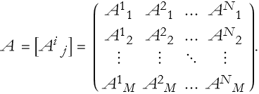
(2.12)

A matrix having one row and N columns, is a row matrix,

(2.13}

A matrix having M rows and a single column, is a column matrix,

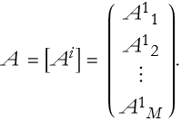
(2.14)

A matrix having the same number of rows and columns is called an N × N square matrix.

For the exercises that follow we will use the following matrices:

If two matrices, say O and P, have the same elements then they are equal and we write O = P.

We can add two matrices by adding their elements,

(2.15)

In order to add matrices the matrices must be of the same order, another word for this is conformable.

Exercise 2.4: Add matrix A to the matrices B through F.

We can also subtract two conformable matrices by subtracting their elements,

(2.16)

Exercise 2.5: Subtract the matrix A by the matrices B through F.

We can multiply a matrix by a number, say a, by multiplying each element by a,

(2.17)

The number a is often called a scalar for historical reasons. The operation described in Equation (2.17) is called scalar multiplication. The operation of addition, subtraction, and scalar multiplication form the nucleus of matrix arithmetic.

The following rules apply, first addition is commutative,

(2.18)

Addition is associative,

(2.19)

There is an additive identity, in this case it is a matrix all of whose elements are 0, we will label this script 0, ,

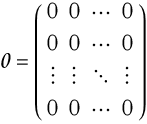
(2.20)

This is called the null matrix. The additive identity is then,

(2.21)

There is an additive inverse,

(2.22)

Scalar multiplication is right-distributive,

(2.23)

Scalar multiplication is left-distributive,

(2.24)

If we have a sum, it can be burdensome to write it out every time, instead of writing

(2.25)

we can instead use the upper-case Greek letter sigma, Σ, to denote the sum. Further, below the sigma we will write the summation variable (the variable that informs us as to what we are summing over), and above the sigma we will place the maximum m value of the summation variable. We will write Equation (2.25) this way,

(2.26)

This is called the summation notation, and it is used throughout mathematics and science.

Given two matrices, R and S, where R is an M ×N matrix and S is an N × T matrix the matrix product of the two is

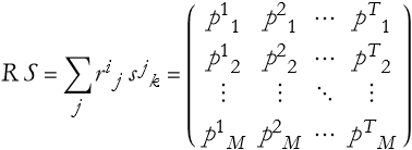
(2.27)

where i=1,…,M, j=1,…N, and k=1,…,T. Where the elements are a set of sums of products,

(2.28)

Assuming all matrices are conformable, then the matrix product is left- and right-distributive and associative

(2.29)

(2.30)

(2.31)

In general, the matrix product is not commutative. In general, O P=, does not imply that either O= or that P=. In general, A B=A C does not imply that B=C.

Exercise 2.6: Multiply A and the matrices B through K and then reverse the order of multiplication in each case.

We now introduce five important kinds of matrices. A square matrix with all off-diagonal elements zero, and all diagonal elements non-zero is called a diagonal matrix. A diagonal matrix whose diagonal elements are all 1, is called the identity matrix, and is denoted I. A square matrix whose elements satisfy the condition , is called an upper triangular matrix. A square matrix whose elements satisfy the condition , is called a lower triangular matrix. Another way of defining a diagonal matrix is that it is both upper and lower triangular.

If O P=I=P O, then P is the inverse matrix of O, . We also note that . Similarly . In general, for a 2 × 2 matrix

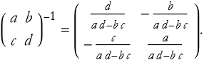
(2.32)

Exercise 2.7: Find the Inverse matrices of  A through F.

A matrix that is the interchange of rows and columns of another matrix is the transpose of that other matrix. We denote this with a T superscript,

(2.33)

The following rules hold.

(2.34)

(2.35)

(2.36)

(2.37)

Exercise 2.8: Find the Transpose of the matrices A through K.

A matrix equal to its transpose is called symmetric, . A matrix equal to its negative transpose is called skew-symmetric, .

2.5 Determinants

A determinant is a special kind of expression that takes a matrix and converts it into a scalar. We will begin with notation, the determinant of a matrix, A is denoted either det(A), or . So, what is a determinant? We will begin with the simplest matrix,

(2.38)

then the determinant is said to be of first order and is written,

(2.39)

This is an interesting result, but not very revealing.

Instead, let’s increase the order of our matrix, and look at an arbitrary 2×2 matrix

(2.40)

this determinant is said to be of second order,

(2.41)

We can see how this structure comes about be examining the array, see Figure 2.23,

Figure 2.23: Evaluating a second-order determinant.

here you can see that the first term in (2.41) is given by multiplying the diagonal elements of the array from the upper + side. The second term in (2.40) is given by subtracting the diagonal terms from the upper - side, then keeping the negative sign, thus we subtract the second term.

This gives us a better clue about how to proceed. We can extend this to an arbitrary 3×3 matrix,

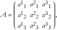
(2.42)

then the determinant is,

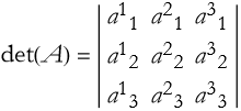
(2.43)

We can look at the array and see geometrically how we should combine the elements, see Figure 2.24

Figure 2.24: Finding the first positive term in a third-order determinant.

here we have the first positive term, . We can also construct the next positive term, see Figure 2.25

Figure 2.25: Finding the second positive term in a third-order determinant.

we have . We can then construct the final positive term, see Figure 2.26

Figure 2.26: Finding the third positive term in a third-order determinant.

we have . We can do a similar construction with the arrows beginning on the - side extending to the + side.

Exercise 2.9: Draw the three diagrams showing this extension from the - to the + side, thus showing what the three negative components of the determinant are.

The end result will look like this,

(2.44)

If we stare at this long enough we will eventually realize that we can factor it.

(2.45)

Something interesting is happening here. If we convert the differences into lower-order determinants,

(2.46)

The first term is acquired by eliminating the row and column indicated from det(A) by the factor, in this case row 1 and column 1. the second determinant is gained by eliminating row 1 and column 2, and the final by eliminating the row 1 and column 3.

Here we note that we have made three submatrices whose determinants are of order -1 from the order of the original matrix. Such a determinant is called a minor of the element , where we have eliminated row i and column j. We can denote the minor as .

If we consider the sign of the minor, then we can define the cofactor of the element as,

(2.47)

We can use the cofactors to calculate the determinant, for the jth row,

(2.48)

for the ith column,

(2.49)

These are called the Laplace expansions, named for the mathematician Pierre Simon Laplace.

Exercise 2.9: Find the determinants of the matrices A through F.

2.6 Arrows

We have seen that physical quantities can be represented by numbers. There is another kind of physical quantity that has not only a magnitude (or number) associated with it, but also a direction. Such a quantity can be represented as an arrow. The simplest such quantity, as we have already seen, is the position of some point with respect to a reference point. The distance between the points would be the magnitude, but it also requires a direction. In this way we can represent a position as an arrow leading from the reference point to the location we are considering. See Figure 2.27.

Figure 2.27: The position arrow.

By convention we denote the arrow for position as r with a little arrow over it, .

The first thing that you can do with such an arrow representation is multiply it by a number. If the number we choose is greater than 1 then the length of the arrow will increase. If the number we choose is both greater than 0 and less than one then the length of the arrow will get shorter. If the number we choose is zero, then the arrow vanishes. If the number chosen is less than zero then the arrow will point in the opposite direction to our original arrow. Thus multiplication by a number other than 1 changes the scale of the arrow. Such numbers are often called scalars. This operation is often called scalar multiplication (this is not to be confused with the scalar product, we will get to that a bit later). This is very similar to the scalar multiple we saw when we studied matrices. Note that the name scalar comes from the Latin word scalaris, this is itself an adjective of the word scala, meaning ladder; this is the basis for the English word scale.

If position can be represented by an arrow, how about a distance interval? It seems reasonably clear that distances can change with a change of scale. For example, if we double the length of our distance scale the distance interval will be multiplied by a half. We call such a contrary relationship is called contravariant. By this we mean that a change in scale produces a contrary change in length.

Exercise 2.10: Graphically multiply some arbitrary arrow by 2, 4, and 1/2.

Exercises 2.11: Can you think of any reason why you couldn’t multiply a position arrow by any real scalar?

Exercises 2.12: Is scalar multiplication of an arrow commutative?

Say we want to add two arrows together. What does it mean to add to ? See Figure 2.28

Figure 2.27: The arrows and .

First we lay down , as in Figure 2.28,

Figure 2.28: The arrow .

Then we place at the head of , as in Figure 2.29.

Figure 2.29: The arrow , placed at the head of arrow .

We can then draw a new arrow from the tail of to the head of . That new arrow is the sum . See Figure 2.30.

Figure 2.30: The sum of the arrows is the new arrow .

Subtraction can be viewed as adding the reversed arrow, (see Figure 2.31).

Figure 2.31: The difference of the arrows is the new arrow .

Exercise 2.13: Is arrow addition commutative?

When we move we travel an interval of distance Δ r in an interval of time Δ t.

What about adding distance intervals? Do those intervals add like arrows? It seems completely reasonable. If we look at our example above, if were to represent the distance between two points and the distance between the head of and some other end-point, then the sum of the arrows would be the distance between the tail of and the head of .

So it seems reasonable that distance intervals can be represented by arrows. In fact such arrows are given a special name, we call such an arrow a displacement.

The speed of travel is then defined as the quotient of the displacement and the time-interval.

(2.50)

Can we represent this quantity by an arrow? It seems obvious that since displacements are contravariant, then so will speed be contravariant. What about addition of arrows, do speeds add like arrows, too? What would that mean. Looking at our example above, if represents the speed of our object, then what are we adding to it to get another arrow?

One possible answer is that the motion could be occurring on a moving platform. If represents the speed of the platform, then the sum is the speed that would be measured by an outside observer.

So speed can be represented by an arrow. In fact we no longer call that arrow representation speed, we call it velocity. Speed is the magnitude, or length, of a velocity arrow.

What happens when you do a push-up? You lift yourself up by pushing against the floor or ground. This push changes our state of motion. We begin at rest, apply the push and we move up. Gravity pulls us down and we stop moving when the push due to our arms matches the pull due to gravity, or we have just pushed ourselves up to the limit of our arm length. So a push changes our state of motion. We call such a push, or pull, a force.

Can we represent a force as an arrow? Let us examine our push-up example. When we begin we are at rest. At this time the only force experienced is that of the floor keeping us from falling down. Thus there is an arrow pointing up that represents the force due to the floor, what we call the normal force, we can denote this . See Figure 2.32.

Figure 2.32: The normal force.

As we exert a downward force, denoted , there are two possible cases based on a sum of the forces used to make the push-up successful .

(2.51)

To examine this, we abstract this diagram to what we call a free-body diagram. We represent the body being acted on by the forces as a point and we draw the force arrows from that point. See Figure 2.33.

Figure 2.33: Our first attempt at a free-body diagram.

This is kind of silly, it implies that if we push hard enough, our arms will sink into the floor. It turns out that Sir Isaac Newton wrote a law of motion that famously has it that, “Every force exerted by some object on a body results in an equal, but opposite force being applied to the object.” So as we push downward on the floor, the floor pushes upward against us, this is what allows us to lift up from the floor. In reality the free-body diagram looks like Figure 2.34.

Figure 2.34: Our second attempt at a free-body diagram.

This too is a bit strange. What is stopping us from floating arbitrarily into the air? We left out the force pulling us down by gravity, . The new free-body diagram looks like Figure 2.35.

Figure 2.35: Our final, correct, attempt at a free-body diagram.

What are the two cases we spoke of? If , then we lift ourselves up. If , then we remain laying on the floor. So, we can see that forces add like arrows.

Exercise 2.14: Is a force arrow contravariant?

Let’s say we have a box, see Figure 2.36.

Figure 2.36: A box.

If we rotate this, the angle of the rotation can be seen as a magnitude. If we choose a right or left rotation, this gives us a direction. So it seems like we might be able to represent a rotation by an arrow.

If we rotate this by 90° to the left about the vertical axis, we get Figure 2.37.

Figure 2.37: Rotating our box by 90° to the left about a vertical axis.

If we then rotate this about 90° to the left about the horizontal axis the figure looks the same as in Figure 2.36.

If we take the original figure and rotate 90° to the left about the horizontal axis, then we get Figure 2.38.

Figure 2.38: Rotating our box by 90° to the left about a horizontal axis.

Then we add a rotation of 90° about the vertical axis it looks the same as in Figure 2.38. Adding the two rotations in opposite order does not give us the same answer. So rotations cannot be represented by arrows. Thus, not every directed magnitude can be an arrow.

2.7 Introducing Vectors

How do we apply a numerical procedure to arrows that represent physical quantities? One answer is to superimpose a coordinate system over the arrow. Let’s say we have the arrow , as in Figure 2.39.

Figure 2.39: The arrow .

Now we can choose the tail of the arrow as the origin of out coordinate system, as in Figure 2.40.

Figure 2.40: Embedding the arrow into a Cartesian plane.

We can apply perpendicular lines connecting the head of to the x and y axes, as in Figure 2.41.

Figure 2.41: Establishing the coordinates of the head of the arrow .

In this way we have the distances along each axis, and . These are called the components of the vector for the coordinate system.

This leaves us with two numbers. We can make a special column matrix,

(2.52)

Such a symbol takes on the label of column vector. In more advanced studies it is also called a tangent vector. From this we can conclude that every arrow is a column vector, or just a vector.

Exercise 2.15: Extend (2.52) to thee-dimensions.

Multiplying a column vector by a scalar is the same as multiplying an arrow by a number

(2.53)

Please note that the Greek letter alpha, α, is different than the a.

Exercise 2.16: Extend (2.53) to thee-dimensions.

Adding column vectors is the same as adding arrows.

(2.54)

Exercise 2.17: Extend (2.54) to thee-dimensions.

2.8 Vector Spaces and Vectors

We can formalize the idea of a vector by defining a set denoted by a double-struck V, V, as being made of a collection of objects, , , and so on. For now we will not name these objects other than to call them elements of V. We can add the elements , and we can multiply the elements by a scalar, . We call the set V a vector space if the following tests are all true:

We can define a rule to add any pair of the elements.

We can define a rule to multiply any element by some scalar.

The operation of addition or scalar multiplication results in another object of the set. Another way of saying this is that the proposed vector space is closed under the operations of addition and scalar multiplication.

The addition of elements is commutative. For example, .

The addition of elements is associative. For example, .

There exists a null element, , such that .

For every, , there exists an additive inverse element, such that, .

Scalar multiplication is associative, .

Scalar multiplication is right-distributive, .

Scalar multiplication is left-distributive, .

Should the set successfully pass all of these tests, then it is called a vector space and all of its elements are renamed to be vectors. Thus the null element becomes the null vector, and the additive inverse element becomes the additive inverse vector.

Exercise 2.18: If you add arrows, is the result always another arrow?

Exercise 2.19: If you multiply a scalar by an arrow, is the result always another arrow?

Exercise 2.20: Is arrow addition commutative?

Exercise 2.21: Is arrow addition associative?

Exercise 2.21: Is there a null arrow? What is the relevance of your answer to Apprentice Exercises 2.18 and 2.19?

Exercise 2.22: Is there an additive inverse arrow?

Exercise 2.23: Is scalar multiplication of arrows associative?

Exercise 2.24: Is scalar multiplication of arrows right-distributive?

Exercise 2.25: Is scalar multiplication of arrows left-distributive?

If you did these correctly, you should conclude that the set of all arrows forms a vector space and that the arrows may be termed vectors. This is very important, many physics books conclude that vectors are arrows, when the correct interpretation is that arrows are vectors, but so are many other things, as we are about to see.

Exercise 2.29: Prove that square matrices of a given order form a vector space. What does this imply about square matrices of a given order?

Exercise 2.30: Prove that the set of third order polynomials of the form also form a vector space.

Exercise 2.31: Prove that the set of third-order column matrices (or column vectors) form a vector space. We have already seen this space and we called it the Euclidean space and denote it .

Any subset S of a vector space that is also a vector space is called a subspace of the vector space. The intersection of any number of subspaces of a vector space is also a subspace of the vector space.

We will have a special vector for every existing vector, say , whose length is one unit along the direction of that vector. Such a vector is called a unit vector. We denote a unit vector by the symbol for the unit vector in the direction of the vector .

If we superimpose a coordinate system over the space we are working in with a number of axes equal to its order, we can establish a unit vector for each of those axes. For Cartesian coordinates in three dimensions we could label them or for the first axis, or for the second axis, and or for the third axis. The set of all relevant unit vectors for the axes are renamed as basis vectors.

If a set of vectors can be written as a sum of products of coefficients and their relevant basis vectors

(2.55)

we call this a linear combination.

2.9 Scalar Products

There are three ways of multiplying two vectors. The second two methods are a bit harder to grasp and we will discuss them in later chapters. We will now examine the first way to do this, whose answer is a scalar. Thus, we call this a scalar product. This is sometimes called a dot product (and we will see why in a moment). We denote this with a dot between the vector symbols. Thus the scalar product of and is denoted .

Before we move on it is time to introduce some more notation. The magnitude of the vector is written . We can define the scalar product for two vectors in a traditional way, assuming we know the angle between them, θ.

(2.56)

Exercise 2.32: What is the scalar product of and if and and θ is ?

The magnitude (or norm) is the length of a vector.

(2.57)

From this we can better define the unit vector

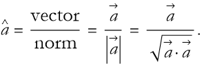
(2.58)

Say that we have two vectors, and that are perpendicular as in Figure 2.42.

Figure 2.42: Two perpendicular vectors.

If we add them we get the traditional sum of vectors as in Figure 2.43.

Figure 2.43: The sum of the two perpendicular vectors.

If we look at this long enough, it will occur to us that this forms a right triangle. We can treat the two vectors, and , as the base and altitude of the triangle and the hypotenuse is . If we apply the Pythagorean theorem, we can write,

(2.59)

We can rewrite this,

(2.60)

If the two vectors are not perpendicular then our diagram changes as in Figure 2.44.

Figure 2.44: The sum of the two non-perpendicular vectors.

Then (2.59) is no longer , but is some correction from ,

(2.61)

We can add a new vector to and we will call it , as in Figure 2.45.

Figure 2.45: Introducing .

The new altitude vector will be renamed , as in Figure 2.46.

Figure 2.46: Introducing .

We then rewrite (2.59)

(2.62)

If we use the Pythagorean theorem for the smaller triangle ,

(2.63)

We can now rewrite (2.61)

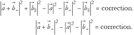
(2.64)

It turns out that the magnitude of a sum of vectors is

(2.65)

so (2.64) becomes

(2.66)

By using the definition of the scalar product we are left with

(2.67)

So what is this correction? It must depend on the angle between the vectors. When  vectors are perpendicular this correction has a value of 0. Can we think of a value of an angle whose value is 0 when the angle is π/2 radians? One comes to mind, cos(π/2)=0.

The vector is called the projection of the vector onto the direction of the vector . How do we find θ? Starting from (2.56)

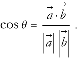
(2.68)

So,

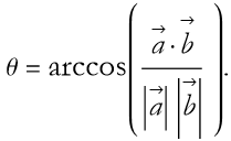
(2.69)

If we have two column vectors, how do we find their scalar products. Say we have two arbitrary column vectors,

(2.70)

then the scalar product is

(2.71)

It turns out that the scalar product of parallel vectors is 1, and the scalar product of orthogonal vectors is 0.

Exercise 2.33: Explain why the scalar product of parallel vectors is 1, and the scalar product of orthogonal vectors is 0.

So the scalar product becomes

(2.72)

For n-dimensional vectors we can generalize it,

(2.73)

Exercise 2.34: What is the scalar product of and if and ?

It can get tiring to write the summation symbols all the time. We will adopt the Einstein summation convention, yes it is named after that Einstein, where any term that has the same superscript and subscript is assumed to be summed over all of the dimensions of the space. Thus,

(2.74)

To apply this to the scalar product we introduce a new symbol,

(2.75)

This is the Kronecker delta, named after Leopold Kronecker. In fact, one definition of the scalar product of two unit vectors is the Kronecker delta

(2.76)

We can now redefine the scalar product.

(2.77)

If we apply the Einstein summation convention, this becomes

(2.78)

Exercise 2.35: Assuming that we stay in three dimensions, thus n=3, calculate the following: , , , and .

There is a second product of vectors whose result is a vector, thus it is called the vector product. We will get to that a bit later. A third product of vectors results in a kind of matrix representation that is called a dyadic product, or a tensor product, we will get to this later.

For Further Reading

Leonard Susskind, George E. Hrabovsky, (2013), The Theoretical Minimum, Basic Books. Chapter 2 is a subset of this chapter.

John Roe, (1993), Elementary Geometry, Oxford University Press. This is one of my favorite books on geometry. The material of this chapter could be expanded into the first five chapters of Roe’s book.

George E. Owen, (1964), Fundamentals of Scientific Mathematics, Harper & Row (reprinted in 2003 by Dover Publications). This is a fantastic little book. It is not a good textbook as it has no practice problems, but it is a nice read and covers the material of this chapter in greater depth in chapters 1 and 2.