Chapter 1: The Nature of Classical Physics

1.0 The First Question

What is the nature of classical physics? By classical physics we mean physics that does not include the actions of the observer (some device or effect that is measuring something—like you) in what is being observed (an experiment or natural phenomena). There are two points of view for classical physics, the first is that of the isolated objects (mechanics), the second is that of things that are everywhere that can influence an item (field theory). This book is mostly about isolated items.

The job of classical mechanics is to predict the future of isolated objects. The great eighteenth century physicist Pierre-Simon Laplace laid it out in a famous quote:

We may regard the present state of the universe as the effect of its past and the cause of its future. An intellect which at a certain moment would know all forces that set nature in motion, and all positions of all items of which nature is composed, if this intellect were also vast enough to submit these data to analysis, it would embrace in a single formula the movements of the greatest bodies of the universe and those of the tiniest atom; for such an intellect nothing would be uncertain and the future just like the past would be present before its eyes.

1.1 Why Classical Mechanics?

Classical mechanics is the basis of all of physics. This is not simply because it describes the behavior of familiar objects, but also because it provides the framework through which all of the rest of physics is presented. The principles by which all natural systems evolve are essentially the same set of rules, in a more abstract and general setting, as those that describe the motion of a simple object experiencing some interaction.

In order to understand the properties of these rules, such as the law of the conservation of energy, we must study them in their abstract forms. In order to make the predictions required of classical mechanics we must first develop the rules of mechanics, put them into a useful mathematical or computational language—what we will call a formulation, then apply the rules of mathematics and/or computation to deduce the outcome of the application of the formulation to a particular situation—what we call a model. It is a model that allows us to make predictions. Predictions are then matched against observations or experimental results. If the model is good at making predictions, then we gain faith in its abilities.

1.2 What is a Particle?

The idea of a particle is an abstraction. Let’s say you want to study the motion of a car. There are the components of the engine moving and exchanging fluids, the wheels rotating and bending, people inside the car moving and breathing, the car itself moving on the road and creating turbulence in the air as it passes. This is a very complicated system.

Imagine that you can zoom out so that you can avoid most of this complexity. You no longer see the internal workings of the car. You have the same system, but it's a simpler picture.

Imagine that you zoom out till all you see is a speck in the distance. This speck still has all of the properties of the car that we started with. All of the internal systems are still there. We just don't need to worry about them.

Now we have to make a leap of faith. We have to believe that we can treat an object as if we were zoomed out till we can treat it as if it were a speck. Think about what we are losing by treating the object as a speck. The first thing we lose is all of the internal complexities of the object. We also lose the size and shape of the object. Whenever we have an object where we do not need to worry about its size, shape, or its internal workings we can look at it as if it were a speck. Such a simplified object is called a particle. The highest level of abstraction for an object of any kind is to treat it as if it were a particle, even though we know that no object is really a particle.

The drawback is that by removing the complexities you also remove levels of reality. So what is the point of the abstraction? It makes the problem simple enough to start analyzing it. Once you understand the simplified problem, you can begin to put the complexity back to make it more realistic. This process of abstraction is the heart of theoretical physics.

1.3 Simple Dynamical Systems and State Space

We will adopt, for the purpose of this chapter, a set of laws of nature that are of the most primitive kind—knowing that we are not considering the real natural laws. These simple laws will act on the most primitive systems we can imagine.

We will begin by stating that in classical mechanics time evolves smoothly and can be represented by any real number. Smoothness is a property that allows one value to smoothly change into the next without a break, we use the mathematical term continuous to describe this property. The property of being continuous is called continuity. Whenever we speak of any real number, what we mean is the totality of the real numbers as a collection, we call such a collection a set. If we denote the set of all real numbers with the symbol double-struck R, R, and we can write time with the symbol, t, as an element of the set of real numbers; we write this symbolically, t∈R. We also note that in classical mechanics time is the same everywhere.

For now, we will assume that we can measure time only in discrete steps. We begin a step at some initial time, , and end at some later time, . This is what we call a time interval, and denote that with the symbol Δ t. This does not mean that we multiply Δ and t, the Δ symbol represents a change in the symbol that follows it, in this case t. Thus Δ operates on t, and we can call it a the increment operator. The combination Δ t is thus considered to be a single symbol,

So we have a stroboscopic world where we can only see what is happening after some interval of time.

A set of particles is called a system. A system that is either the entire universe or is so isolated from everything else that it behaves as if nothing else exists is a closed system.

Here we have the first of a series of exercises. I advise you strongly to try each exercise, because we can only really learn by doing things. Don’t worry if you get the answer wrong, that is how we learn. We don’t really learn anything by being right, unless you figure out the right answer as you go. There are three kinds of exercises: Apprentice Exercises are those that are either very important, or they are laid out in a way that carefully describes each step. I recommend spending no more than five minutes on such exercises, if you don’t get it then set it aside for a day and come back to it while you continue reading ahead—this time spending up to ten minutes on it, if you don’t get it set it aside again and then spend up to fifteen minutes the next day, and so on for as much as a week—if you don’t get it by then you can email me and I (or a colleague who has gotten it) will try to help you.  Journeyman Exercises are those where I leave most of the details up to you, for these I recommend spending up to fifteen minutes on the first try. Master Exercises are a brief description of a personal research project for you to perform—this may include problems that have not yet been solved or where a lot of work has been done, but more can be added. Such problems are open ended and may have no set time frame.

Apprentice Exercise 1.1: Since the notion is absolutely important to theoretical physics, think about what a closed system is and speculate on whether closed systems can actually exist. What assumptions are implicit in establishing a closed system? What is an open system?

If we know everything about a system so that we can completely characterize it, then we say that we know its state. Each fact that we know is a variable that characterizes the state, and we call it a state variable. The number of values required for each state variable is the number of degrees of freedom for the system.

The set of all states that a system can be in is what we call the system’s state space. The state-space is not necessarily ordinary space; it’s a mathematical set whose elements label the possible states of the system.

The simplest system I can think of is very boring, one where nothing ever changes—there is only one possible state. This is called a static system.

A simple system that is a little more interesting is one with two possible states. An example of such a system is a coin, and it can be in one of two states: heads or tails. Another example is a light switch, it can be on or off.  Figure 1.1 illustrates a two-state space.

Figure 1.1: The state space of a system having two states.

The big question becomes, “In our stroboscopic world, how does a system change in one time interval?” The answer is that we need some rule to tell us what state the system can be found in as we pass from one time interval to the next. Such is system is said to evolve in time. A system that evolves over time is called a dynamical system. The rules that govern such changes are often referred to as dynamical laws. Applying a dynamical law in the state space diagram will be represented by including an arrow from one state to the next.

One possible law is that everything stays the same. If the dynamical system begins in State 1 it stays there, and the same for State 2. We can make a state space diagram of this (see Figure 1.2).

Figure 1.2: A law of dynamics for a two-state system.

We can write these dynamical laws in equation form. Such an equation is often called an evolution equation. Our system has one degree of freedom which we can denote by the letter s. Our letter s has only two possible values; s=-1 and s=+1, respectively for States 1 and 2. We also use a symbol to keep track of the time intervals. Here we have a discrete evolution in intervals of time. Instead of writing Δ t we will use the letter n. The state at the time interval n is described by the symbol s(n), this stands for the value of s at the time interval n.

Let's write the evolution equation for our dynamical law. This dynamical law says that no change takes place. In equation form, we write this

In other words, whatever the value of s at the nth step, it will have the same at the next step. This forms a sequence of values, the length of the sequence is the number of time intervals that we allow to pass. We will learn more about sequences in the next chapter.

Another possible dynamical law is in Figure 1.3; where we begin in one state and the system shifts to the other state.

Figure 1.3: Another dynamical law for a two-state system.

The evolution equation for this second dynamical law has the form

Once we know the initial state of the system, we can predict how the dynamical system will evolve for every time interval after that. We call such a law deterministic.

One way to become more generalized is to increase the number of states. Let’s say that we have six possible states (see Figure 1.4).

Figure 1.4: A six-state system.

We could invent something called Dynamical Law 1 (see Figure 1.5).

Figure 1.5: Dynamical Law 1.

We can imagine another law, Dynamical Law 2 (see Figure 1.6).

Figure 1.6: Dynamical Law 2.

Dynamical Law 2 is really not all that different than Dynamical Law 1, each state has an arrow that leads to a unique state, and none are left out. Dynamical Laws 1 and 2 both endlessly repeat their patterns; this is called a cycle.

Apprentice Exercise 1.2: Draw a state space diagram with three states. Then connect the states by arrows. Do this for four states as well.

Apprentice Exercise 1.3: Redraw the states in Dynamical Law 2 so that they look like the order of states in Dynamical Law 1. In this way you have shown that the two systems are equivalent under a transformation of states.

You can also have qualitatively different laws. Dynamical Law 3 has two cycles (see Figure 1.7).

Figure 1.7: Dynamical Law 3.

Figure 1.8 shows Dynamical Law 4 with three cycles.

Figure 1.8: Dynamical Law 4.

It will take a long time to write out all of the possible dynamical laws for a six-state system.

Journeyman Exercise 1.4: Can you think of a general way to classify the laws that are possible for a 6-state system?

Dynamical Laws 1 through 4 are all  deterministic into the future. It is important to note that they are also deterministic into the past. These are the ideal sort of laws governing the evolution of dynamical systems in physics. The fact that they are deterministic into the past is a property that we call reversibility, and we say that such laws are reversible. As such these are all good prototypes of what we call laws of physics.

No real situation is so well defined. The simple aspects of dynamical laws get jumbled up in complexities. Despite such complexities any classical dynamical system will be deterministic—but you must know every last detail to see this.

What kind of dynamical laws are not allow? We have a dynamical system with three possible states, 1, 2, and 3, and a dynamical law represented in Figure 1.9.

Figure 1.9: A system that is irreversible.

This is completely deterministic into the future. It is not reversible; suppose you are at State 2, where did you come from? You could come from either 1 or 3, and there is no way to tell for sure. We call this situation irreversible, since we cannot run the law backwards.

Say we have the same state space as the last one, but with all arrows reversed as in Figure 1.10.

Figure 1.10: A system not deterministic into the future.

Here we are reversible, but not deterministic; if you are at State 2 where do you go from there? The law fails to tell you how to proceed.

Both of these laws fail to be either deterministic or reversible. They are forbidden in physics. To be allowable at any given state there must be one arrow in, to tell us where we came from, and one arrow out, to tell us where we are going. This can be called the law of conservation of information.

1.4 Using Number Systems in Physics

There is no reason why you can’t have a dynamical system with an infinite number of states. We could say that there is a state for every integer. Here we recall that the set of integers is a mathematical structure denoted with the double-struck Z, Z. If we label our states m, then we would write m∈Z, saying that any given state label is some integer (see Figure 1.11).

Figure 1.11: State space for an infinite system of integers.

A simple dynamical law for such a system is that we shift one state in the positive direction at each time interval (see Figure 1.12).

Figure 1.12: A dynamical rule for a an infinite system.

This is allowable as each state has one arrow in and one arrow out. Infinity is not a number, it is a place-holder. We can easily express this rule in the form of an equation:

Apprentice Exercise 1.5: Determine which of the following four dynamical laws are allowable:
s(n+1)=s(n)-1 .
s(n+1)=s(n)+2 .


Draw a diagram for each dynamical law.

We can add more states and dynamical laws to this dynamical system. We can say that we are separating the state space into regions (see Figure 1.13).

Figure 1.13: Separating an infinite system into regions.

If we start with a number, then we just keep proceeding through the set of integers. On the other hand, if we start at A or B then we cycle between them. So, we can have a mixture of regions, one where we cycle around in some states, while in others we move off to infinity.

1.5 Cycles in State Space

Let’s consider a system with three regions. States 1 and 2 each belong to one cycle, while 3 and 4 belong to the third (see Figure 1.14).

Figure 1.14: Separating the state space into regions.

Whenever a dynamical system breaks the state space into such separate regions there is the possibility of keeping a memory of where we started, Such a memory is a conservation law; telling us that something is kept intact for all time. Let’s say that states 1 and 2 represent the value of a variable, we could relabel them +1 and -1. We also have a cycle between States 3 and 4, where both states have a value of 0. (see Figure 1.15).

Figure 1.15: Replacing the labels with specific values.

Since the dynamical law does not allow you to jump from cycle to cycle, that is a conservation law, since starting at one value means you have that value forever.

As stated above, this can be called information conservation. Information conservation is probably the most fundamental aspect of the laws of physics. Why is that so? We don't really know why the laws of physics have the properties that they have. All we have is the experimentally derived fact that the laws of physics are information conserving.

1.5 The Theory of Distances

We must be able to locate a particle. To that end we state these facts:

We will understand that everything is happening in a place. We will call this place a space. We have already seen state spaces.

Our space can have regions within it that we will call subspaces. Each such subspace can be thought of as a state.

One class of such subspaces has no size or shape, this is called a point.

Given the fact that the point has no size or shape, and a particle is considered without regard to size or shape, we can say that a point is a mathematical structure that can describe the location of a particle.

This reduces our problem to finding a point representing the location of a particle within a space. The first thing to realize is that we cannot find the position of anything without knowing what that position is relative to. In other words, we have to identify some arbitrary reference point. We will call this reference point O. This is the classical notation for the origin. You can think of the origin as a place to start. We can also set a point representing the location of the particle, called P (see Figure 1.16).

Figure 1.16: The origin and the location of a particle.

We now recall from basic geometry Euclid's First Postulate: For every point O and every point P not equal to O there exists a unique line ℓ that passes through O and P. This line is denoted .

Any two points, O and P, and the collection of all points between them, that lie on the line combine to form a line segment. Our segment is denoted (Figure 1.17).

Figure 1.17: The line segment .

The segment   is called the distance between O and P. We can measure this distance, denoted D(OP).

Recall that, given a number x the absolute value of x is x itself so long as x is greater than or equal to 0; if x is less than 0 then its absolute value is -x. Symbolically we write it this way:    

The Ruler Axiom states: Given a line ℓ, there exists a one-to-one correspondence between the points lying on the line ℓ and the set of real numbers such that the distance between any two points on ℓ is the absolute value of the difference between the numbers corresponding to the two end points. This is another way of stating that there is a distance interval. From this we can construct another expression for distance by applying the definition of the absolute value to the Ruler Axiom and then to the definition of distance we get,

To measure this we have to establish a unit of length. Let us say that this is a segment bounded by the points and (see Figure 1.18).

Figure 1.18: Applying a unit length segment.

We next have to find a point on such that 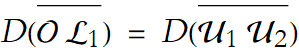(see Figure 1.19),

Figure 1.19: Finding the point .

If we repeatedly apply something, we call it an iteration. We apply the unit length iteratively until we have n equal segments 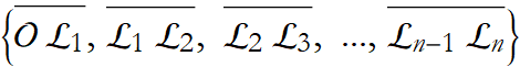(see Figure 1.20).

Figure 1.20: Finding the successive points.

And thus the distance for the segment is then,

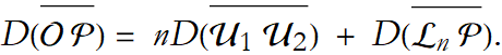
Thus, measuring distance is the iterative application of a unit of length n times and then adding any fractional remainders.

We can't discuss a practical measurement without including the unit of measurement we are using. In this way the length of the segment becomes an algebraic quantity with the number of units being the coefficient of the symbol for the unit. We might say four feet, or ten point three six meters, or six and a half light years, etc.

In the abstract we can assume that we are talking about arbitrary units, and so will implicitly understand that units are being considered without stating it.

1.6 Units of Measurement

As we have seen we need a unit of measurement for distance. We also need a unit of measurement for time intervals.

There are many sets of units for measurement. We will discuss the three most commonly used. The first is the English system (which is, ironically, only used by the United States), the International System (also called the metric system, or the SI System), and what we will call the cgs system (a factor of the metric system).

Lengths in the English System are in inches (abbreviated in), feet (12 inches, abbreviated ft), yards (3 feet, abbreviated yd), and miles (5,280 feet or 1,760 yards, abbreviated mi). Time is measured in seconds (abbreviated sec), minutes (60 seconds, abbreviated min), and hours (60 minutes, abbreviated hr).

Lengths in the SI System are in meters (about 1.1 yards, abbreviated m). Time is measured in seconds.

Length in the cgs System is in centimeters (1/100 meters, abbreviated cm). Time is measured in seconds.

1.7 The Variability of Measured Data

Position is represented by a real number, we write x∈R. The problem is that almost all real numbers can only be written as decimal approximations. Thus there is some uncertainty as to exactly where a particle is located. We also gain some error in the measurement process itself, we almost never have a perfect fraction of a unit when we measure something. We can only approximate such a position. This is what we call measurement error.

This uncertainty in measurement will adversely influence any prediction made by a dynamical law as you evolve the system in further time intervals. In this way, a small uncertainty in a measurement can be magnified as time goes on, this is called the propagation of error. For this reason, in practice, classical systems are not really endlessly predictable. All we can do is say that for some number of time intervals the system is deterministic.

Let's say that I want to predict where every molecule of gas in the room is going to go next, ignoring quantum mechanics. It turns out that there is a certain degree of precision in the information we can have at any instant of time that will allow me to extrapolate such positions out to a particular time. Any given level of precision will not allow me to extrapolate positions beyond a certain number of time intervals. Beyond that the errors grow out of control. If I want to predict how things will behave at longer times I will have to do better in the precision of my statement of the initial state of the dynamical system.

So, in practice, the idea of determinism is defective because to predict out to a certain time we need a level of precision that is better than anyone can really achieve. Theoretically it is deemed possible, in classical physics, to achieve such a level of precision to be deterministic. In reality it is impossible.

Some systems are very predictable for a number of intervals. Other systems are not so predictable, they get out of control after a very few intervals of time and are called chaotic. The principles are the same for both, the only difference is the level of precision you need to extrapolate out to a given time.

Another way of stating this is that the equations allow for infinite predictability given infinite precision in stating the initial state of the system.

1.8 What is Motion?

Any change in the location of an object in a corresponding interval of time is motion. There is only one thing wrong with this; we do not know what is meant by change.

Part of determining position is to measure the distance from the origin to the object. Once we know the distance to the particle then we need to determine the direction. The traditional way is to choose an arbitrary reference line as 0° and then measure the angle counterclockwise from the 0° line (Figure 1.21).

Figure 1.21: Locating the particle.

We traditionally write this angle using the Greek letter theta, θ. In physics we use the radian instead of the degree as a measure of angle. We say that there are 2 π radians in 360°, or 1radian=360°/(2 π)≈57°, thus 90°=π/2, and 30°=π/6.

Once we have measured both the length and angle of the segment we call that a directed line segment. A directed line segment is an example of a mathematical structure called a vector. In this case we have a specific type of vector called a position vector. A position vector is classically denoted by the symbol r. Writing it by hand you might use either a half arrow over the top of the vector or a tilde under the vector . We will use a full arrow above a symbol to denote a vector, thus we write the position vector, . Motion can be thought of as a change in the position vector in any corresponding time interval.

1.9 The Myth of Scientific Laws

We have stated that for a dynamical law to be considered a physical law it must be both deterministic and reversible. But what is a law of physics? How does it come about? What makes it a law?

When we collect data for some phenomena we use mathematical techniques to attempt to find patterns in that data. We assign a mathematical structure to this pattern that makes sense. Such a perceived pattern is not considered a fact. We then examine other related data to see if that pattern exists there, too. If the pattern exists in every case we examine we develop a level of confidence in it, and consider it to be a fact. That pattern, assuming it is both deterministic and reversible, is written in the form of a mathematical rule and is often called a law of physics.

Let’s say that you have been thinking about gases. You read up on it and have identified some physical quantities that you can represent using numbers and units. We can define a gas as a substance that fills the entire volume it sits in. We know that volume is measured in cubes. In the English system we use cubic inches (denoted ), cubic feet (denoted ), and so on. In the SI system we use the cubic meter (written ). In the cgs system we use the cubic centimeter (written either cc or ), equivalently it can be called a milliliter (written as ml).

You can say that if the gas is pushing against any surface it has a pressure, denoted P. Pressure is a force (what is pushing) divided by the area of the surface over which it pushes. In English units forces are measured in poundals (denoted pdl), in SI this is measured in Newtons (denoted N), and in cgs it is measured in dynes (denoted dyn).

You also note that a gas will have a temperature. The temperature of something is more than just a reading on a thermometer. It measures the average energy in something based on the vibrations of the atoms that make up the substance. Of course, we don’t really know what energy is. For now we can consider it as what we read on a thermometer. In the English system we use degrees Fahrenheit (denoted °F). In the SI system and cgs system we use degrees Centigrade (or Celsius, both written °C).

You then think about the relationship between the pressure, the volume, and the temperature of a gas. After a while you become so curious that you do some experiments and measure the pressure of a gas for different volumes at constant temperature. You find that the pressure, symbolized by P is proportional to the inverse of the volume, symbolized by V, and proportionality is symbolized by ∝. Then we write this relationship symbolically,

After some more analysis we note that (Equation 1.8) is exactly true when the volume is multiplied by some constant, determined by the gas under study. We will symbolize this constant c, so we have,

We can rewrite this,

This is called Boyle's law, it is named after Robert Boyle, who confirmed its validity in 1662 It is one of the basic laws describing the behavior of gases.

All such laws are similar in two ways. First, they are similar in that they are all true within what I will call their region of applicability, that is when the assumptions that were made when they were discovered are still valid. Second, they all break down in some way when those assumptions are no longer valid. In other words when the law is used outside of its region of applicability it is no longer valid. The message is then that these laws are not laws at all, they are observed patterns that we have a lot of faith in.

So, is physics just a collection of such laws? No, such a collection is an absolute statement of fact and is unable to extend itself beyond the regions of applicability of the laws. Such a list of laws fails to explore the relationships between the various laws in the list. Additionally, and even more importantly, we do not know all of the laws of physics, so no such list can ever be thought of as complete.

Does this mean that physical laws should not be considered? No, it means that we must be aware of the regions of applicability of the laws we want to use, and we must be aware that we don’t know them all.